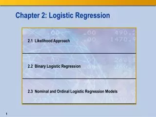
Chapter 2: Logistic Regression

1. Chapter 2: Logistic Regression

2. Chapter 2: Logistic Regression

3. Objectives • Explain likelihood and maximum likelihood theory and estimation. • Demonstrate likelihood for categorical response and explanatory variable.

4. Likelihood • The likelihood is a statement about a data set. • The likelihood assumes a model for the data. • Changing the model, either the function or the parameter values, changes the likelihood. • The likelihood is the probability of the data as a whole. • This likelihood assumes independence.

5. Likelihood for Binomial Example • The marginal distribution of Survived can be modeled with the binomial distribution.

6. Maximum Likelihood Theory • The objective is to estimate the parameter and maximize the likelihood of the observed data. • The maximum likelihood estimator provides • a large sample normal distribution of estimates • asymptotic consistency (convergence) • asymptotic efficiency (smallest standard errors)

7. Maximum Likelihood Estimation • Use the kernel, the part of the likelihood function that depends on the model parameter. • Use the logarithm transform. • The product of probabilities becomes the sum of the logs of the probabilities. • Maximize the log-likelihood by finding the solution to the derivative of the likelihood with respect to the parameter or by an appropriate numerical method.

8. Estimation for Binomial Example

10. 2.01 Multiple Choice Poll • What is the likelihood of the data? • The sum of the probabilities of individual cases • The product of the log of the probabilities of individual cases • The product of the log of the individual cases • The sum of the log of the probabilities of individual cases

11. 2.01 Multiple Choice Poll – Correct Answer • What is the likelihood of the data? • The sum of the probabilities of individual cases • The product of the log of the probabilities of individual cases • The product of the log of the individual cases • The sum of the log of the probabilities of individual cases

12. Titanic Example • The null hypothesis is that there is no association between Survived and Class. • The alternative hypothesis is that there is an association between Survived and Class. • Compute the likelihood under both hypotheses. • Compare the hypotheses by examining the difference in the likelihood.

13. Titanic Example

14. Uncertainty • The negative log-likelihood measures variation, sometimes called uncertainty, in the sample. • The higher the value of the negative log-likelihood is, the greater the variability (uncertainty) in the data. • Use negative log-likelihood in much the same way as you use the sum of squares with a continuous response.

15. Null Hypothesis using the marginal distribution

16. Uncertainty: Null Hypothesis Analogous to corrected total sum of squares

17. Alternative Hypothesis using the conditional distribution

18. Uncertainty: Alternative Hypothesis

19. Uncertainty: Alternative Hypothesis Analogous to error sum of squares

20. Model Uncertainty Analogous to model sum of squares

21. Hypothesis Test for Association

22. Model R2

24. 2.02 Multiple Answer Poll • How does the difference between the – log-likelihood for the full model and the reduced model inform you? • It is the probability of the model. • It represents the reduction in the uncertainty. • It is the numerator of the R2 statistic. • It is twice the likelihood ratio test statistic.

25. 2.02 Multiple Answer Poll – Correct Answer • How does the difference between the – log-likelihood for the full model and the reduced model inform you? • It is the probability of the model. • It represents the reduction in the uncertainty. • It is the numerator of the R2 statistic. • It is twice the likelihood ratio test statistic.

26. Model Selection • Akaike’s Information Criterion is widely accepted as a useful metric in model selection. • Smaller AIC values indicate a better model. • A correction is added for small samples.

27. AICc Difference • The AICc for any given model cannot be interpreted by itself. • The difference in AICc can be used to determine how much support the candidate model has compared to the model with the smallest AICc.

28. Model Selection • Another popular statistic for model selection is Schwartz’s Bayesian Information Criterion (BIC). • It measures bias and variance in the model like AIC. • Select the model with the smallest BIC to minimize over-fitting the data. • It uses a stronger penalty term than AIC.

29. Hypothesis Tests and Model Selection This demonstration illustrates the concepts discussed previously.

31. Exercise This exercise reinforces the concepts discussed previously.

33. 2.03 Quiz • Is this association significant? Use the LRT to decide.

34. 2.03 Quiz – Correct Answer • Is this association significant? Use the LRT to decide. • It is not significant at α=0.05 level.

35. Chapter 2: Logistic Regression

36. Objectives • Explain the concepts of logistic regression. • Fit a logistic regression model using JMP software. • Examine logistic regression output.

37. Overview

38. Types of Logistic Regression Models • Binary logistic regression addresses a response with only two levels. • Nominal logistic regression addresses a response with more than two levels with no inherent order. • Ordinal logistic regression addresses a response with more than two levels with an inherent order.

39. Purpose of Logistic Regression • A logistic regression model predicts the probability of specific outcomes. • It is designed to describe probabilities associated with the levels of the response variable. • Probability is bounded, [0, 1], but the response in a linear regression model is unbounded,(-∞,∞).

40. The Logistic Curve • The relationship between the probability of a response and a predictor might not be linear. • Asymptotes arise from bounded probability. • Transform the probability to make the relationship linear. • Two-step transformation for logistic regression. • Linear regression cannot model this relationship well, but logistic regression can.

41. Logistic Curve • The asymptotic limits of the probability produce a nonlinear relationship with the explanatory variable.

42. Transform Probability • Step 1: Convert the probability to the odds. • Range of odds is 0 to ∞. • Step 2: Convert the odds to the logarithm of the odds. • Range of log(odds) is -∞ to ∞. • The log(odds) is a function of the probability and its range is suitable for linear regression.

43. What Are the Odds? • The odds are a function of the probability of an event. • The odds of two events or of one event under two conditions can be compared as a ratio.

44. Probability of Outcome Total 80100180 Probability of not defaulting=60/80 (.75) in Group A Probability of defaulting=20/80 (.25) in Group A

45. Odds of Outcome Odds of Defaulting in Group A probability of defaulting in group with history of late payments probability of not defaulting in group with history of late payments ÷ 0.25÷0.75=0.33 Odds are the ratio of P(A) to P(not A).

46. Odds Ratio of Outcome Odds Ratio of Group A to Group B odds of defaulting in group with history of late payments odds of defaulting in group with no history of late payments ÷ 0.33÷0.11=3 Odds ratio is the ratio of odds(A) to odds(B).

47. Interpretation of the Odds Ratio no association B more likely A more likely 0 1 ∞

49. 2.04 Quiz • If the chance of rain is 75%, then what are the odds that it willrain?

50. 2.04 Quiz – Correct Answer • If the chance of rain is 75%, then what are the odds that it willrain? • The odds are 3 because the odds are the ratio of probability that it willrain to the probability that it will not, or 0.75/0.25=3.