Download
1 / 38
390 likes | 438 Vues
Explore the concepts of genotypic and allele frequencies, Hardy-Weinberg equilibrium, external forces on genetic populations, and the effects of mutation, migration, and selection on gene pools. Discover how gene flow and speciation influence genetic diversity.

E N D
Definitions • Population: a group of interbreeding individuals • Genotypic frequency: The frequency of a specific genotype in a given population (AA, Aa, aa) • Allele frequency: The frequency of a specific allele within a given population • Gene pool: The collective gene frequencies of a specific population
Genetic variation • Changes in the DNA sequence of a gene produce genetic variation. • Experiments indicate all natural populations contain a great deal of genetic variation.
Genotype and allele frequencies • Genotype and allele frequencies are the “genotype” of a population. • Frequencies of three genotypes: AA (100) Aa (250) aa (50) f(AA) = #AA/total = 100/400 = .250 (P) f(Aa) = #Aa/total = 250/400 = .625 (H) f(aa) = #aa/total = 50/400 = .125 (Q)
Allele frequencies • Allele frequencies are used to describe populations. • Frequencies of alleles of one gene: AA (100) Aa (250) aa (50) p = f(A) = (2AA + Aa)/ 2total = (200 + 250)/800 = .5625 q = f(a) = (2aa + Aa)/ 2total = (100 + 250)/800 = .4375 p + q = 1
Hardy-Weinberg Law • Assumptions: • Infinitely large population • Random mating • No mutation, migration, selection • In an ideal population the allele and genotype frequencies do not change from generation to generation. • The genotype frequencies can be described by the equation: p2 + 2pq + q2 = 1
Using Hardy-Weinberg • Is the following population in Hardy-Weinberg equilibrium? • MM 345 MN 490 NN 165 (1) What are the allele frequencies? (2) What are the expected genotype frequencies? (3) Is the difference significant?
Another example: An population starts with 250 MM and 150NN individuals, what will be the genotype and allele frequencies at equilibrium? • Allele frequencies = p = f(M) = q = f(N) = • Genotype frequencies = p2 = 2pq = q2 = • In a population of 1000 individuals how many will be of each genotype? MM = MN = NN =
Calculation of allele frequenciesof recessive traits • The allele frequency can be calculated using • the fraction of homozygous recessive individuals in the population. • Example: • Albinos are present in the population at a frequency of 1 in 20,000. What is heterozygote frequency? • q = 1/20,000, therefore q = 1/141 • p = 140/141 • heterozygous = 2(1/141 x 140/141) = 1/71 • 1/71 x 1/71 x 1/4 = 1/20,000, therefore most • births are from matings of heterozygous. 2
External forces can affect Hardy-Weinberg equilibrium • A Hardy-Weinburg equilibrium population has no mutation, migration, sampling error (genetic drift), or selection. All of these can change the allele frequencies in the next generation. • How do these forces change allele frequencies, and which have major effects on real populations?
Mutation • Mutations are the source of new alleles. • p = frequency of A q = frequency of a • A -> a = forward mutation, rate = u • a -> A = reverse mutation, rate = v up = number of new a alleles vq = number of new A alleles • p = vq - up, q = up - vq
Migration: gene flow Population 1 f(A) = p1 • Natural populations are not closed. • Migration between two populations can change allele frequencies. • ex. (A)p1 = 0.8, (A)p2 = 0.5 migration from p1 to p2 produces a new population with p3 = mp1 + (1-m)p2 • What is p3 if m = 0.2? m Population 3 m f(A) = p1 Population 2 f(A) = p2 1-m f(A) = p2
The new frequency is: p3 = mp1 + (1-m)p2 p3 = 0.2 (0.8) + (1- 0.2) 0.5 = 0.56 • The rate of change depends on the rate of mating between p1 and p2. • Migration eventually produces new equilibrium allele frequencies if random mating occurs between the two populations.
Gene Flow • Gene flow distributes new alleles throughout the population. • Restricting gene flow can lead to formation of new species.
Speciation • Mechanisms that block gene flow are reproductive isolating mechanisms (RIM). • RIMs lead to genetically distinct subpopulations. • Accumulation of enough genetic differences produces new species. • RIM may be genetic (inversions, translocations) or physical.
Selection • Natural or artificial selection results from differences in reproductive fitness. • All organisms produce more offspring than survive • Organisms differ in their ability to survive • Favored genotypes are selected and reproduce Direct selection of a bacterial strain for antibiotic resistance is an example of survival of mutant offspring. Similarly, diploid organisms can be selected for by the presence of insecticides, fungacides, etc. The selective disadvantage of a disfavored genotype is called the selection coefficient, and varies from 0 to 1, where 1 represents the most disfavored. Fitness varies from 1 to 0, where 1 represents the most fit.
Hbs • In an area of high malaria infestation the heterozygotes for Hbs have a selective advantage. • The frequency of Hbs is high in areas where malaria is common.
Selection can change a population very quickly, and can maintain a recessive lethal allele at high frequencies. Allele Freq. Genotype Frequencies HbA Hbs HbAHbA HbAHbs HbsHbs p0 .99 .01 .98 .02 .0001 p1 .91 .09 .83 .16 .008 p2 .67 .33 .45 .44 .11 p3 .55 .45 .30 .50 .20 p4 .53 .47 .28 .50 .22
Neutral Alleles • If an allele is selectively neutral, it’s frequency will change by chance from generation to generation.
Genetic Drift leads to fixation • Genetic drift can lead to fixation of one allele. • 400 populations of 8 individuals, with a = 0.5 and A = 0.5. Most populations were fixed for one allele after 32 generations.
Inbreeding co-efficiency • Defined as the percentage of homozygousity due to common ancesters • Brother and sister mating ¼ • First cousin 1/16
Problem • A recessive genetic disease happens around 1/1,000,000. What will be the disease frequency for a first cousin marriage?
Analyzing the quantitative variation of multifactorial traits
Quantitative traits • Continuous traits (quantitative) individuals vary in the quantity of the characteristic. ex. Length of ear in corn. ex. Height in humans • Discontinuous traits (qualitative) individuals have qualitative phenotypic differences. ex. Eye color in Drosophila: white vs red. ex. Seed shape in peas: round vs wrinkled. • Quantitative traits show a characteristic, Non-Mendelian pattern of inheritance.
Qualitative (Mendelian) Quantitative • Are quantitative traits controlled by Mendelian genes? P X X F1 F2 3/4 1/4
Nilsen Ehle: polygenic hypothesis • Red kernel wheat crossed with white kernel produces an intermediate F1. • The F2 show a range of colors. • Conclusion: color is a polygenic trait. P X F1 F2 1/64 6/64 15/ 64 20/64 15/64 6/64 1/64
Phenotypes for quantitative traits are measured in populations • Samples are taken from a population. • The phenotype of each individual in the sample is measured. • The results can be shown as a frequency distribution. Fig 5.6
Describing a quantitative trait • Phenotype is measured in terms of the mean and variance of the frequencyx/n • variance = S2= V = a numerical measure of the range: (x - x)2 n - 1 • standard deviation = s = V
Analysis of Variance • The variance is equal to the sum of its components. • The phenotypic variance of a quantitative trait has two components: Vp = Vg + Ve phenotypic variance = genotypic variance + environmental variance.
Heritability • h2= heritability = VG / Vp Heritability indicates how much of the variance is caused by genetic differences.
Examples of heritability organism trait Heritability Humans stature 0.65 IQ 0.7 - .80 Cattle milk yield 0.35 body weight 0.65 pigs back-fat thickness 0.70 poultry egg weight 0.50 egg production 0.10 frog size 0.69 development rate 0.31
Selection for a trait in a population • Repeated selection for a specific phenotype in a population is possible if genetic variation exists, and the trait is governed by multiple genes.
Selection differential and response to selection • Heritabity can be calculated from selection experiments: Selection response (R) = h2 X selection differential (S)
X P O R s h2 = R/S X = old population P = parents O = offspring
Heritability can be calculated from selection experiments • Ex. Two fish with a length of 25 cm are crossed. These are from a population with a mean length of 16 cm. • The F1 have a mean length of 22.8 cm. • What is h2 for this trait in this population? • S = selection differential = • R = response to selection = • h2 = 16 25 22.8 R s
Heterosis Parents X X • Hybrid corn was first utilized in the early part of the last century. Corn yields have gone from 40 bu/acre to 140 bu/acre. • Four highly inbred lines are crossed, and the two hybrids are crossed to give a double cross hybrid. X Single cross hybrid Double cross hybrid