Modeling the Vibrating Beam
This study presents a model explaining the vibrations of a horizontal beam influenced by a small voltage application. Utilizing a spring-mass model, parameters were optimized to accurately depict the beam's behavior. The analysis revealed useful confidence intervals and highlighted challenges in model fitting, such as residual dependencies and normality assumptions. Despite the limitations, the model has potential applications in fields such as bridge construction, aerospace, and diving board design, paving the way for future enhancements and more robust modeling approaches.


Modeling the Vibrating Beam
E N D
Presentation Transcript
Modeling the Vibrating Beam By: The Vibrations SAMSI/CRSC June 3, 2005 Nancy Rodriguez, Carl Slater, Troy Tingey, Genevieve-Yvonne Toutain
Outline • Problem statement • Statistics of parameters • Fitted model • Verify assumptions for Least Squares • Spring-mass model vs. Beam mode • Applications • Future Work • Conclusion • Questions/Comments
Problem Statement GOAL IDEA Develop a model that explains the vibrations of a horizontal beam caused by the application of a small voltage. Use the spring-mass model! Collect data to find parameters.
Solving Mass-Spring-Dashpot Model The rod’s initial position is y0 The rod’s initial velocity is yo
Statistics of Parameters • Optimal parameters: C= 0.7893 K=1522.5657 • Standard Errors: se(C)=0.01025 se(K)= 0.3999 • Standard Errors are small hence we expect good • confidence intervals. • Confidence Intervals: • (-1.5892≤C≤-.7688) • (-1521.76≤K≤-1521.7658)
Confidence Intervals • We are about 95% confident that the true value of C is between .8336 and .8786. • Also, we are 95% confident that the true value of K is between and 1523 and 1527.8. • The tighter the confidence intervals are the better fitted model.
Sources of Variability • Inadequacies of the Model • Concept of mass • Other parameters that must be taken into consideration. • Lab errors • Human error • Mechanical error • Noise error
Fitted Model • The optimal parameters depend on the starting parameter values. • Even with our optimal values our model does not do a great job. • The model does a fine job for the initial data. • However, the model fails for the end of the data. • The model expects more dampening than the actual data exhibits.
C= 1.5 K= 100 C= 7.8930e-001 K= .5226e+003 Through the optimizer module we were able determine the optimal parameters. Note that the optimal value depends on the initial C and K values.
Least-Square Assumptions • Residuals are normally distributed: • ei~N(0,σ2) • Residuals are independent. • Residuals have constant variance.
Residuals vs. Fitted Values • To validate our statistical model we need to verify our assumptions. • One of the assumptions was that the errors has a constant variance. • The residual vs. fitted values do not exhibit a random pattern. • Hence, we cannot conclude that the variances are constant.
Residuals vs. Time • We use the residuals vs. time plot to verify the independence of the residuals. • The plot exhibits a pattern with decreasing residuals until approximately t= 2.8 s and then an increase in residuals. • Independent data would exhibit no pattern; hence, we can conclude that our residuals are dependent.
Checks for normality of residuals! Residuals are beginning to deviate from the standard normal!
QQplot of sample data vs. std normal • The QQplot allows us to check the normality assumptions. • From the plot we can see that some of the initial data and final data actually deviate from the standard normal. • This means that our residuals are not normal.
The Beam Model This model actually accounts for the second mode!!!
Applications • Modeling in general is used to simulate real life situations. • Gives insight • Saves money and time • Provides ability to isolating variables • Applications of this model • Bridge • Airplane • Diving Boards
Conclusion • We were able to determine the parameters that produced a decent model (based on the spring mass model). • We did a statistical analysis and determined that the assumptions for the Least Squares were violated. • We determined that the beam model was more accurate.
Future Work • Redevelop the beam model. • Perform data transformation. • Enhance data recording techniques. • Apply model to other oscillators.