Slavery in the Ancient World
330 likes | 734 Vues
Slavery in the Ancient World. Bob Allen Nuffield College, Oxford 2008. Slave mode of production. Second stage in Marxist scheme Slavery was extensive in ancient world, at least in some times and places Athens in 5 th and 4 th century BC

Slavery in the Ancient World
E N D
Presentation Transcript
Slavery in the Ancient World Bob Allen Nuffield College, Oxford 2008
Slave mode of production • Second stage in Marxist scheme • Slavery was extensive in ancient world, at least in some times and places • Athens in 5th and 4th century BC • Italy during expansion of Roman Republic and the Empire • Slaves may have amounted to one third of the population in these areas but little exact information. • Slaves worked in mining and agriculture as well as domestic service.
Character of slavery varied. • In Athens and Roman Republic, the main source of slaves were captured either in war or bought from victors in other wars and raids. • In agriculture and mining, treatment was extremely harsh, sex ratios unbalanced, families not allowed. • Slaves revolts were one result.
Supply of captive slaves declined as imperial expansion slowed and then receded.
When expansion slowed, slaves were bred. • Estates were reorganized and slaves became Servi casati. • Slaves allowed to have houses and families. • They grew their own food on their own plots. • Slavery came to look a lot like medieval serfdom.
Slavery often assumed to inhibit economic growth. • This view was propounded most famously by M.I. Finley in many works. • Slavery was a pre-capitalistic system of organization. • Governed by custom and coercion rather than economic incentives. • Absence of a labour market emblematic of limited role of markets in general.
Questions about ancient slavery: • Why was it so extensive? • Why did its organization change? • What was its impact on economic growth? We have already seen some standard answers to these questions.
We will re-examine these issues using the cliometric methods developed to study American slavery. • In early modern period, about 12 million Africans taken to the Americas to work in plantations. • About 500,000 of these were in the United States where they cultivated cotton and other crops.
Character of slavery depended on the supply of slaves. • When slaves were imported freely (and cheaply), slavery was exceptionally harsh. • Slave trade abolished in the British Empire in 1807 and in the US in 1808. • Afterwards, American slave owners encouraged high fertility. • US slavery abolished during civil war in 1860s.
An old tradition maintained: • Slavery was economically irrational. • Slavery inhibited economic growth. • Slavery was unprofitable and unviable, so it would have died out without the Civil War. • These issues were addressed in a great research trajectory featuring Conrad & Meyer (1958), Yasuba (1961), Fogel & Engerman (1974), and other works.
The historian Ulrich Phillips (1905) argued that slavery was not viable. • Slavery was only established because wages were very high. • Slave labour was unproductive and worth using only when slaves could be cheaply imported. • After the abolition of the slave trade, slave prices rose relative to cotton prices, and that meant that slavery was not profitable. • Slaves were kept only as status symbols—not because they were economically valuable.
These claims were supported by calculations like these by Sydnor (1933). from: R Fogel & S Engerman, Reinterpretation of American Economic History, p. 321.
Weaknesses in the calculation: • Deducting interest as a cost. • Eliminating that expense raises profit rate to 8.4% • What Snydor calculated was the rate of pure profit, which was positive and equivalent to 8.4% > 6%. • Not including the value of slave children as a benefit. • Treating the investment as lasting forever and deducting depreciation to make it finite may introduce errors if the depreciation is not consistently measured.
One of the first papers of the ‘new economic history’ was Conrad and Meyer’s calculation of slavery profitability (1958). • Separate calculations for males and females. I only consider males here. • 20 year old male slave cost $1450. • Cost per year of maintaining him was $20.50. • Output per slave was 3.75 bales (500 lbs each) per year. • Price of cotton was $0.067 per pound, so annual revenue per slave was $125.625.
We can compute the rate of return: Slave price = ∑ (annual revenue-annual cost)/(1+i)ⁿ where summation is from n = 1, 2, 3,…..T 1425 = ∑ (125.625-20.50)/(1+i)ⁿ where summation is from n = 1, 2, 3,…..35 (ages 20 to 55) Now solve the equation for i!
Enter the data in Excel and use internal rate of return function: This rate of return was the same as railway bonds, which shows that slavery was profitable.
The situation was more complex: • Since the slave trade was illegal, the supply of slaves was fixed, and their price was demand determined. • The demand price of slaves was the present values of their net income. • The Conrad-Meyer calculation simply shows that slave income was discounted at the railway bond rate.
Slave price = ∑ (annual revenue-annual cost)/(1+i)ⁿ where summation is from n = 1, 2, 3,…..T Substituting $1425 for slave price and solving for i = 6.25% gives Conrad and Meyer rate of return. But slave price was set in market by discounting annual net income with i = .0625. Slave price = ∑ (125.625-20.50)/(1+.0625)ⁿ where summation is from n = 1, 2, 3,…..35
Yasuba (1961) pointed out that viability was different from profitability. • Viability meant that it was profitable to breed slaves. • If slavery was viable, the price of the adult slave was greater than the future value of the cost of rearing him or her. • Alternatively, slavery was viable if the present value of all net revenues from birth to death was greater than zero. • The difference, in either case, was the ‘capitalized rent,’ and positive capitalized rent indicates viability. • Yasuba did calculations that are hard to reproduce that show that American slavery was viable.
We can do some of these calculations with ancient data to address the questions about ancient slavery. • Was it profitable to purchase a slave in the Roman empire? This throws some light on the question of the ‘customary’ nature of the economy. • Was it profitable to breed slaves in ancient Athens? How about the Roman Principate? This throws light on how the expansion of the empire affected the character of slavery.
Rate of return to buying a slave, 1st century AD(Conrad and Meyer calculation)
The rate of return of 9.1% looks plausible. • Net income is the difference between the annual earnings of a free labourer and the cost of maintaining a slave • Most foundations realized 6% on capital, but a few realized 12%. • Slave pricing looks economically rational. • This counts against Finley view that the economy was customary.
A Yasuba viability calculation explains the hutting of slaves. • In 5th century BC Athens and the Roman Republic, slaves were very cheap because there were so many captives. • The price was so low that it was not profitable to breed slaves. • Slavery was ‘not viable’ in Yasuba terms. • The situation was different as the supply of captives declined in 1st century AD. • Then the price of slaves exceeded the cost of rearing them, and slavery was ‘viable’. • Hence, servi casati
We need a life table for this (West level 2, female, exp at birth = 22.5 years)
We also need: • Interest rate (6%) since future value of a cost is: FV = cost per year * (1 + i)ⁿ where n is years to 15 • Cost per year worked out from cost per calorie per adult and calorie requirement of each age. • Cost of breeding a 15 year old is sum of the FV of the costs for the 15 years: • Cost of 15 year old= ∑(cost/yr)*(1+i)ⁿ,n=1..15
Was breeding profitable? • Not in the age of conquests when slaves were cheap: The cost of breeding a 15 year old was 296 drachmas > the price of 125-150 drachmas • Yes after the Roman Empire was established and stopped expanding. The cost of breeding was 355 denarii < the price of 500-600 denarii • Simple economics explains the change in the character of Roman slavery.
Why was slavery viable?The Malthusian context • In the case of breeding, the subsistence income of the slave is the subsistence for a family. • This is the same amount as the subsistence wage that would prevail if the population was in a ‘Malthusian equilibrium’. • Possible exceptions or slippage? • Slavery based on breeding new slaves is only viable if the wage is above subsistence (an Engerman point). • Slavery was viable in the Roman empire because the economy generated a high standard of living. This ties in with modern reassessments of the performance of the Roman economy and challenges the Finley view.
In the case of slavery based on captives, • The system could persist even if the wage was at ‘subsistence’. • ‘Subsistence’ in this sentence means subsistence for a family. • Since the slaves are not expected to reproduce in the captive system, the income of the slave is only enough to support a single individual. • This is about one third of the ‘subsistence’ for a family.