Optimising Explicit Finite Difference Option Pricing For Dynamic Constant Reconfiguration

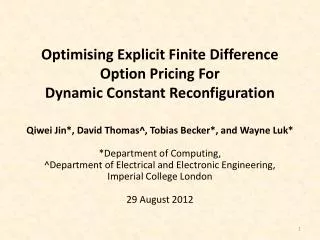
1. Optimising Explicit Finite Difference Option Pricing For Dynamic Constant Reconfiguration Qiwei Jin*, David Thomas^, Tobias Becker*, and Wayne Luk* *Department of Computing, ^Department of Electrical and Electronic Engineering, Imperial College London 29 August 2012

2. Contributions 1. Novel optimisation for Explicit Finite Difference (EFD): • preserves result accuracy • reduces hardware resource consumption • reduces number of computational steps 2. Two approaches to minimise: • hardware resource utilisation • amount of computation required in the algorithm 3. Evaluation: 40% reduction in area-time product • 50%+ faster than before optimisation • 7+ times faster than static FPGA implementation • 5 times more energy efficient than static FPGA implementation

3. Background • Financial put option • gives the owner the right but not the obligation to sell an asset S to another party at a fixed price K at a particular time T • Explicit Finite Difference (EFD) Method • useful numerical technique to solve PDEs • used for options with no closed-form solution • Discretises over asset price space (S) and time (t), and maps them onto to a grid

4. Background • The Black Scholes PDE and the EFD grid

5. Background • The entire EFD grid • updated from right to left, backwards in time t • updated by a stencil with coefficients α, β and γ Z=lnS, κ≡(S, K , r, T, σ)

6. Background • Stencil computation mapped to FPGA (Static)

7. Background • Dynamic constant reconfiguration$ • reduce area, power and improve performance Constant multipliers, reconfigure to update (Dynamic) $ “Dynamic Constant Reconfiguration for Explicit Finite Difference Option Pricing”, Becker et. all

8. Two Optimisation Methods Two methods to optimise high performance designs • Use custom data formats* • to reduce area • preserve sufficient result accuracy • Use constant specialisation and reconfiguration $ • further reduce area and energy consumption • Is there a third method? * “A mixed precision Monte Carlo methodology for reconfigurable accelerator systems”, Chow et. all $ “Dynamic Constant Reconfiguration for Explicit Finite Difference Option Pricing”, Becker et. all

9. 1. Novel Optimisation Method • To obtain the best trade-off: • reduce hardware resource consumption • set the EFD grid carefully • minimise resource usage of constant multipliers • reduce the number of computational steps required in the EFD grid • ensure the result meets the accuracy requirement • avoid unnecessary computation

10. Novel Optimisation Method: Approach • Normalising the option coefficients • fixed point datapaths used instead of floating point ones • less hardware resources consumed • Identifying efficient fixed point constants • yield smaller constant multipliers • adjust the EFD algorithm to make use of them • Reducing number of computational steps • make sure it is smaller than the original and • preserve result accuracy

11. Normalising Option Coefficients • Option descriptor κ≡(S, K, r, T, σ) • Option price f is unbounded • Since 0< K<∞ and 0< S< ∞ • Bits are wasted in fixed point • not all integer bits utilised all the time • κcan be normalised κ’≡(S/K, 1 , rT, 1, σ√T) andf=Kf’ • 0 ≤ f’ ≤1, f’ is bounded • bits are fully utilised

12. 2. Efficient Fixed Point Constants This will be discussed in two parts • Possibility of finding efficient constants • Two approaches to scan the search space • minimise hardware resource utilisation • minimise the amount of computation

13. Possibility of Finding Efficient Constants • Assuming three B-bit fixed point constant multipliers are generated • based on coefficients α, β and γ • each use Nα, Nβ, Nγunits ofresource (i.e. in LUTs) • Nα L, Nβ L, Nγ L • Lis a set containing all possible outcomes of resource consumption of B-bit constant multipliers • NL, the size of L depends on the implementation details of the fixed point library • P(Nα=x)= P(Nβ =y)= P(Nγ =z)=1/ NLwhere x,y,z  L • due to complex optimisation techniques applied • assuming Nα, Nβ, Nγare i.i.d. uniform random numbers in set L

14. Possibility of Finding Efficient Constants • The probability of getting any Nα, Nβ, Nγcombination is (1/ NL)3 • The probability of finding a set of constants which halves the hardware resource is therefore 12.5% or (1/2)3 • The probability to find 20% size reduction is 51.2% or (4/5)3 • It is quite possible to find efficient constant combinations in the search space

15. Efficient Fixed Point Constants • Possibility of finding efficient constants • Two approaches to scan the search space • minimise hardware resource utilisation • minimise the amount of computation

16. Scanning the search space • Coefficients α, β and γare flexible • certain properties must be met • ΔZand Δt determines the coefficients • Grid density can be adjusted • ΔZand Δt determines grid density

17. Simple Example Before After Adjust ΔZ NLUT: 533 NLUT: 335 37% reduction in NLUT result based on flopoco p&r

18. Simple Example β Coefficients Values α Relative Error Relative error γ λ λ = ΔZ/ Δt

19. Minimising Hardware Resource Utilisation • Constants in the form of 2E (E  Z) leads to smaller multipliers • multipliers are implemented by shift operators in fixed point arithmetic • Making α, β and γclose to form 2E • corresponding multipliers likely to be smaller • assuming the hardware resource consumption is related to the hamming weight of the constant

20. Minimising Hardware Resource Utilisation • The coefficients need to meet the following criteria: • α+β+γ=1, α>0, β>0,γ>0 • μ(r, σ, Δt) = μ’(α, β, γ, ΔZ) • mean, 1st moment • Var(σ, Δt) = Var’(α, β, γ, ΔZ) • variance, 2nd moment • Skew = Skew’(α, β, γ, ΔZ) • skewness, 3rd moment • Kurt = Kurt’(α, β, γ, ΔZ) • Kurtosis, 4th moment Statistical Moments should be equal to EFD Moments

21. Minimising Hardware Resource Utilisation • Make the EFD scheme converge • the criteria must be met • A minimisation routine • search around a efficient set of constants • (i.e. α=2E1, β=2E2,γ=2E3 or 0.25, 0.5, 0.25) • force the criteria to be met • first and second moments must match • differences in third and fourth moments minimised • grid convergence is guaranteed

22. Minimising Hardware Resource Utilisation • Pros: • possible to find very small constant multipliers • hardware consumption close to the 2E multipliers • Cons: • has no control over Δt or ΔZ • the EFD problem size can be unbounded • result accuracy is not guaranteed • requires a 2D search space (Δt, ΔZ) • some times not possible in business • Works under assumption • hamming weight is related to hardware resource consumption

23. Efficient Fixed Point Constants • Possibility of finding efficient constants • Two approaches to scan the search space • minimise hardware resource utilisation • minimise the amount of computation

24. Minimising Amount of Computation How much computation is actually needed? Relative error Relative error λ Δt Relative error against Δt and λ, where λ = ΔZ/ Δt

25. Minimising Amount of Computation • Δt is usually determined by business fact (fixed) • i.e. if options are exercised on a daily basis, Δt=1 day β Coefficients Values α Relative Error Relative error γ λ

26. Minimising Amount of Computation • With Δt fixed, find a λ(i.e. ΔZ, since λ = ΔZ/ Δt) • must meet the result accuracy requirement • ΔZ> ΔZtree , amount of computation is reduced • Search in [λ- ε,λ] • ε is a small number • find a set of coefficients with local optimal hardware consumption • result accuracy is guaranteed since relative error grows with λ

27. Minimising Amount of Computation • Pros • amount of computation in the result EFD grid is minimised • Result accuracy is guaranteed • fast search under simple search space (1D), no minimisation routine required • Cons • global optimal is NOT guaranteed

28. 3. Evaluation: Implementation • Xilinx Virtex-6 XC6VLX760 FPGA, ISE 13.2 • FloPoCo library for fixed point datapath • MPFR library for fixed point error analysis • Nelder-Mead multivariable routine in GNU scientific library for minimisation • Place and route results are reported

29. Experiment Setting • 23 bit fixed point number format is used • with 1 bit for integer and 22 bits for fraction • Relative error tolerance is 2E − 4 • compared to double precision result • same level of accuracy is used in industry • Δtis set as 1/365 • Assuming daily observation in a 365-day year • Result compared to our previous work • 23 bit fixed point dynamic designs – unoptimised

30. A Typical Case European option Result from implementations is compared to the Black Scholes formula result κ≡ (S, K, r, T, σ) =(70, 70, 0.05, 1.0, 0.3).

31. P&R Result: 1000 Typical Options Max=906 Max=710 22% Reduction in Upper bound

32. Future Work • Use more sophisticated hardware estimation tools for better result • Generalise the work to support more types of EFD schemes • Long term: address trade-offs • in speed, area, numerical accuracy, power and energy efficiency • for a variety of applications and devices

33. Summary 1. Novel optimisation for Explicit Finite Difference (EFD): • preserves result accuracy • reduces hardware resource consumption • reduces number of computational steps 2. Two approaches to minimise: • hardware resource utilisation • amount of computation required in the algorithm 3. Evaluation: 40% reduction in area-time product • 50%+ faster than before optimisation • 7+ times faster than static FPGA implementation • 5 times more energy efficient than static FPGA implementation