Acknowledgement : Australian Managing Climate Variability Program (MCVP)

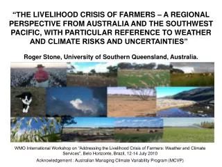
1. “THE LIVELIHOOD CRISIS OF FARMERS – A REGIONAL PERSPECTIVE FROM AUSTRALIA AND THE SOUTHWEST PACIFIC, WITH PARTICULAR REFERENCE TO WEATHER AND CLIMATE RISKS AND UNCERTAINTIES” Roger Stone, University of Southern Queensland, Australia. WMO International Workshop on “Addressing the Livelihood Crisis of Farmers: Weather and Climate Services”, Belo Horizonte, Brazil, 12-14 July 2010 Acknowledgement : Australian Managing Climate Variability Program (MCVP)

3. Outline • Both a detailed analyses - eg: climate and farm cash income + some case study reports and an overview of climate systems affecting this region – (strong ENSO impact). • Focus on aspects associated with extremes of climate variability and how these impact on farmer well-being and livelihood – links to agricultural yield – also vulnerability associated with stocking rates. • Climate variability – yield - farm profit – linking to decisions at a wide range of temporal scales. • Forecasting farm cash income - using key climate indicators – links to seasonal climate management issues – • The sensitivity of farm-cash income to climate variability. • Whole value-chain approaches (farm/mill/transport) valuable in understanding farmer livelihood. • Value in taking an ‘optimality approach’ according to the type of climate decade..

4. In this region, Australia, in particular, has very high year-to-year rainfall variability (100 years of data for Australia and generally also for the other countries) (Love, 2005)

5. And parts of Australia have also long-term shifts in rainfall (mm/decade)

6. 10-year running mean rainfall Rockhampton The relevance of the ‘intersection’ of climate variability and longer-term climate shifts

7. Variability in Australian wheat yield - annual variation in Australian rainfed wheat yield and the SOI (Nicholls).

8. Variation in shire wheat yield (Moree Plains Shire) - stronger relationship in eastern regions - new insurance, derivative products?

9. Cereal yield, climate (growing season rainfall) and farm profit - in southern regions (note the shift to major loss of profits, due to the continued run-down in resources, capital, ‘farmer energy’, income). Motivation by Birchip Cropping Group, Victoria, Australia (courtesy D Rodriguez)

10. The key issue of agricultural management decisions on many scales - and connecting to climate systems on many scales (Meinke and Stone, 2005)

11. AU$50-200K pa AU$200 – 500K AU$100-200K (based on farmer interviews) The costs of inputs – inputs required to make operational and tactical farm management decisions..... BoM Logistics (intra-seasonal, >0.2 years) Sowing / harvesting Application of agrochemicals Tactical (intra-seasonal, 0.2-0.5 years) Crop nitrogen management Crop agrochemicals Tactical (seasonal, 0.5-1 years) Crop type (e.g. wheat or chickpea, maize or sorghum) Marketing (e.g. sell, buy or store) (Rodriguez, 2010)

12. AU$300-500K pa AU$500K – 1M AU$1m-$20m Medium to longer-term farm business planning and climate systems BoM Crop sequences (inter-annual, 1-4 years) Long or short fallows (CI, summer/winter cropping) To irrigate cotton or grains Crop rotations (multi-annual to decadal, 2-10 years) Grains or cotton Cropping or livestock / fodder Transformational (inter-decadal, 10-20 years) Irrigated or dryland cropping Cropping or livestock / fodder Farm investment (storages, land, machinery, etc) Succession planning (Rodriguez, 2010)

13. It possible to forecast farm cash incomes? (in order to develop improved planning strategies or identify those years when government aid may be more in demand) – method is to forecast farm cash income using climate indicators – “probability that simulated farm cash income will exceed the long-term median value” (1900-2003) Based on ABARE’s AgFIRM model for forecasting the impact of climate variability on farm incomes – utilises hindcasting forecasts of crop yields and pasture growth combined with prices available at the end of June to forecast farm incomes for the coming year. Nelson and Kokic, 2004

14. (a) (b) July 2001 July 2002 Strong relationship to the forecast of agricultural commodities: Probabilities of exceeding long-term median wheat yields for every wheat producing shire – July 2001 and July 2002. – combining crop simulation modelling with climate modelling (Potgieter et al)

15. Large variability in farm cash income by ENSO impact Use of AgFIRM to simulate mean farm cash income - Nelson and Kokic, 2004 (Kokic et al. (2004) developed and tested a hybrid modelilng system, the Agricultural Farm Income Risk Model (AgFIRM), that brought together the best available biophysical models of Australian crop and pasture yield, with ABARE’s econometric model of farm incomes. The model provides a capacity to simulate the regional impact of climate variability on farm incomes. It can also provide conditional forecasts of the likely impact of climate variability on farm incomes one year into the future, using well established methods of seasonal climate forecasting.)

16. ENSO/SOI phase probability distributions/boxplots and simulated farm cash income (Nelson and Kokic, 2004)

17. A regional perspective – central NSW – large variability in farm cash income depending on ENSO state Nelson and Kokic, 2004

18. Probability distribution (boxplots) of simulated mean farm cash income by ‘SOI phase’ (Nelson and Kokic, 2004)

19. Sensitivity of farm incomes to climate variability - “The relationship between forecast seasonal conditions and the sensitivity of Australian crop farm incomes to climate variability. “The sensitivity of farm cash income to climate variability is generally lower in years when the SOI phase is ‘consistently positive’ or ‘rapidly rising’ at the end of May and June”. “Conversely, in years when the SOI phase is ‘consistently negative’ or ‘rapid fall; incomes are much more sensitive to climate variability”. This is true even for regions with low income variability such as SW Western Australia and the Eastern Darling Downs”. Nelson and Kokic, 2004

20. Also take an optimality approach according to the type of decade–Example of present farm business position (red dot) and the range of possible outcomes in terms of profit, economic risk and soil loss, for a 2000ha farm-during a ‘dry decade’ (the value of decadal forecasting?) (Cox et al, 2009). Dry decade

21. Optimality Approach – Example of present farm business position (red dot) and the ‘landscape’ of possible outcomes in terms of profit, economic risk and soil loss, for a 2000ha farm -during a wet decade-the value of decadal forecasting? (Cox et al, 2009). Wet decade

22. And…The value of a whole-farm systems approach in linking climate forecasting to farmer’s decisions and operating returns.. Rodriguez et al., 2006

23. Agricultural Production Systems Simulator (APSIM) simulates Assessing likely yields according to decision options -the key value in the linking role of simulation modelling • Provides historical yield of crops and pastures • Assimilates key soil processes (water, N, carbon) • Assimilated surface residue dynamics & erosion • Provides a range of management options • crop rotations + fallowing • short or long term effects

24. APSIM: precise daily time step model that mathematically reproduces the physical processes taking place in a cropping system

25. 6000 5500 5000 4500 4000 Yield (kg/ha) 3500 3000 2500 2000 1500 15-Sep 15-Oct 15-Nov 15-Dec 15-Jan Negative Negative Negative Negative Negative Sow date & SOI Phase “The value of climate forecast information for farming decisions impacts on likely yields – use of Whopper Cropper which utilises pre-run APSIM simulations – examples: When to sow my sorghum crop to achieve the highest potential yield? Effect of sowing date on sorghum yield range at Miles, Southern QLD with a ‘consistently negative’ SOI phase for September/October (Other parameters - 150mm PAWC, 2/3 full at sowing, 6pl/m2, medium maturity. Source; WhopperCropper

26. Cattle industry - insights into management practices leading to producer livelihood vulnerability related to climate variability: • A general over-expectation of safe carrying capacity of stock by farm managers, investors and governments. • Stock numbers, other herbivores (eg rabbits and kangaroos) and, in some cases, woody weed seedlings, increase in response to periods of above-average rainfall that precede drought episodes and thus lead to subsequent high levels of land degradation.

27. Intermittent dry seasons within an otherwise wetter period (decade) result in heavy grazing pressure, damage to the ‘desirable’ perennial species and ultimately the grazing land resource. This leads to the rapid collapse of the land to carry animals at the onset of major drought. • Extreme utilisation in the first years of drought by retaining stock causes further loss of perennial species, exacerbating the drought impacts in subsequent years. • A rapid decline in, or generally low, commodity prices results in some managers retaining stock in the hope of better prices or the fear of a high cost of restocking. • Continued retention of stock through a long drought period compounds damage to the resource and delayed recovery from the drought. • A sequence of drought years results in a rapid decline of surface cover, which reveals the extent of previous resource damage and further accelerates the degradation process, thereby further increasing the vulnerability to subsequent drought (Stone et al., 2003; McKeon et al., 2004).

28. Salinger, 2009.

29. New Zealand issues – case studies

30. NZCase Study One - ‘lack of reliable rainfall in both summer and winter is the biggest climatic challenge’.....’this has become more of a factor in recent years’ ... • El Niño and La Niña events both cause problems.... • the main challenge with unreliable rainfall is that the hills dry out quickly and so farmers try to get rid of their lambs early.... • A downstream consequence of dry summers is poorer lambing percentages.... • Also because of the land committed to pine-trees, most of which was in gorse, and effectively under pressure to reafforest, these farmers do not have any land to fall back on when conditions do get dry...” (Ian and Barbara Stuart - Adapting to climate change in eastern New Zealand”)...

31. Case Study Two - “Carry over effects - key points for the Bay of Plenty region, New Zealand • The carryover effects of the 2007/8 drought - combined with variable weather, including a very dry autumn in 2009, production only recovered partially (up 7 percent compared with 2007/08) to 97 500 kilograms of milksolids. • Reduced payout, down to $5.20 per kilogram of milksolids, net cash income dropped 28 percent to $519 500, compared with 2007/08. • Higher costs and lower payout resulted in a significant cash loss of $53 800 in 2008/09 – • As a result of the combination of losses in 2008/09 and the lower than expected $4.55 per kilogram of milksolids payout in 2009/10, “farmer morale is subdued”.

32. Carry-over impacts on farm profit in New Zealand - Bay of Plenty Region (Courtesy: Ministry of Agriculture and Forestry, 2009)

33. Fiji (Fiji Meteorological Service Headquarters in Namaka, Nadi Airport).. Aspects related to the sugar industry in the overall region -

34. Everingham et al, 2002

35. Climate information application for sustained profitability in the sugar industry – Fiji and Australia (Everingham, et al 2002). Industry Business and Resource Managers Information Axis General Targeted Government • Water allocation • Planning and policy associated with exceptional Events • Crop size • Forecast • Early Season • Supply • Supply Patterns • Shipping • Global Supply • Irrigation • Fertilisation • fallow practice • land prep • planting • weed manag. • pest manag. • Improved Planning for wet weather disruption – season start and finish • Crop size forecast • CCS, fibre levels • Civil works schedule • Land & Water Resource • Management • Environmental Management C l i m a t e forecast information Farm Harvest, Transport, Mill Catchment Marketing Policy Industry Scale Axis

36. Fiji Sugar farmer and miller: case study decisions related to climate in order to improve viability: • Grower decisions: • Land preparation – ‘after the wet spell the land needs to be dry for tractors to move in the field’ – important April onwards... • Seed cane planting – rain necessary for good establishment of cane – important April/May. • Herbicide and fertiliser efficiency is improved if advanced knowledge of weather/climate is known. • Miller decisions: • Mill opening and closing – high value in advanced knowledge • -Eg: high rainfall in May/June and low rainfall in December there is high value in late opening and late closing. • -: low rainfall in May/June and high rainfall in December there is high value in early opening and early closing. • Shipping decisions: • Good knowledge of possible weather conditions can assist in predicting sugar production and thus arrange for shipments in advance (Gawander, 2009).

37. Ways to prevent a crisis? Case study example - better sugar farm management decisions – Farmer Darren Reinaudo, 22 April 2002. • ‘Climate pattern in transitional stage so I keep a watchful eye on the climate updates • I take special interest in the sea surface temperatures (SST) particularly in the Nino 3 region. • There is currently some indications of warming in the Niño 3 region which hints at a possible El Niño pattern developing • Replant would be kept to a minimum • Harvest drier areas earlier, even if CCS maybe effected. • We don’t run the farm based solely on climate information and forecasts, it’s just another tool to consider when making decisions”.

38. Additional factors contributing to livelihood? A wide range of other aspects besides climate - vulnerability exposure variation in Australia for rainfed pasture producing regions, depending on whether a suite of measures are included (left-hand image) (and including such aspects as significant land degradation) or only natural and physical capital is included (right-hand image) (Nelson et al., 2005).

39. Also - the potential for more extreme climate and weather events – further crises for farmers….

40. Intensity of hurricanes according to the Saffir-Simpson scale (categories 1 to 5): 100% increase in Category 5 and Category 4 systems since 1970. P. J. Webster et al., Science 309, 1844 -1846 (2005) ‘Based on a range of models, it is likely that future tropical cyclones will become more intense, with larger peak wind speeds and more heavy precipitation associated with ongoing increases in tropical SSTs’

41. Finally - fisher livelihood? Aspects related to climate ‘drivers’ may also be important. Relationships between Spanner Crab Catch off eastern Queensland and the Nino3 SST (Stone, Meinke, and Williams, 2005).

42. Summary • Overall, high relationship between climate variability (ENSO), yield and farm profit/farm cash income with potential links to crisis periods for producers and farmers– value in linking to decisions at a wide range of temporal scales – and value in forecasting farm cash as well as yield to assist preparedness (by government or farmers). • Climate variability and agricultural yield vary enormously in the region –strong relationship to ENSO and decadal patterns – over expectation of good seasons and thus excessively high stocking rates (cattle) and subsequent poor returns and high land degradation in subsequent drought . • The likely sensitivity of farm cash income to climate variability - generally lower than normal income sensitivity in years when indicators suggest break of El Niño or La Niña pattern at the end of May and June - higher income sensitivity under developing El Niño. • Key aspects related to whole-farm and also whole-industry and value chain – example of sugar industry (eg Fiji).. • Flow on impacts in years beyond major droughts (eg New Zealand)..key aspects of more extreme events impacting on farm viability.

43. Thanks to the following colleagues: • Dr Rohan Nelson (Federal Department of Climate Change), Canberra. • Dr Daniel Rodriguez, Agricultural Production Systems Research Unit (APSRU/DEEDI), (Queensland Government, Toowoomba). • Howard Cox, Agricultural Production Systems Research Unit (APSRU/DEEDI), (Queensland Government, Toowoomba). • Sid Plant, Farmer, Kulpi, Queensland. • Anthony Clark, NIWA, New Zealand.

44. Thank you

46. Best practice in the delivery of seasonal forecasting systems to farmers - the important aspect of co-learning with farmers if we are serious about improving the livelihood of farmers- ‘Participative R&D in action’. Tully Consultative Group sugar/climateproject (Russell Muchow; Yvette Everingham, Roger Stone; CSIRO/JCU/DPI&F/USQ)

47. ? ? Simulated Wheat Yield 1890+ 1.5 5-year running mean - Wentworth, 1884 to 1998 1.0 0.5 0.0 Standard Deviations from the mean -0.5 -1.0 -1.5 1894 1901 1908 1915 1922 1929 1936 1943 1950 1957 1964 1971 1978 1985 1992 Assessing the potential for ‘exceptional drought assistance’ for farmers- use of simulation models to determine the relevance of recent agricultural droughts in an historical context. Simulated Wheat Yield 1950+