Understanding Production Technology, Risk, and Adoption in Agriculture
390 likes | 538 Vues
This document explores the intricate relationships between production functions, input-output processes, and technology adoption in agriculture. It distinguishes between short-run and long-run production functions while considering heterogeneity among producers. The analysis includes risk management, credit constraints, and the process of choosing optimal technologies. It employs a quantitative approach to assess productivity, externalities, and costs associated with various technologies, highlighting the importance of effective input use and technology choices in maximizing agricultural output.

Understanding Production Technology, Risk, and Adoption in Agriculture
E N D
Presentation Transcript
Production technology and risk Ravello David Zilberman
OUTLINE • Production • Adoption and the environment • Risk • Policy
Production functions • They relate input use to output Y=f(X) Y output X vector of input • Varies significantly over spcae and time • Long run production functions- that reflect technology after a period of adjustment are different than short run • Heterogeneity among producers Yi=AiKiaiLibi • Each element fo the production function may vary by individuals- better managers may have a larger Ai (neutral shift) other have better labor or capital productivity. Then there are differences associated with time change
Heterogeneity of quality • Outputs of different quality demand different input use • Inputs’ quality varies-a good worker can produce more • Land quality and exposure to sun may double yields • It is useful to normalize input units-production functions are functions of effective input. Distinguish between applied input (X) and effective input (E) where • E=Xq- where q is an indicator of input use efficiency • Example- X is unit of labor applied by a worker of productivity q If the production function is Y=f(Z) when output is measured in unit of effective inputs, it becomes • Y=f(qX)- and you get less output with a bad worker • Capital good vary in quality because of manufacturer, vintage, past use, etc
Discrete and continuous choices • There may be several alternative technologies- each indexed by i. • Farmers need to make discrete choices- which technologies to use, and • Continuous choices- Allocation of variable input • The land use – in farms land may be used with several technologies- or crop • The allocation question- • Whether to adopt a technology • How much land to allocate • How much variable input to use wit technology
Risk and credit • If farmers are maximizing profit or expected utility • Farmers may diversify land among technologies • Because of risk aversion reasons • Credit constraint • Labor constraint ( Seasonality) • We will stat with case of risk neutral farmer and look at adoption choices • Then move to diversification
How to analyze adoption choices?- a multistage process • Need to choose • Whether to adopt a technology • How to use it optimally- the decision process • Quantify each of the technologies- in terms of productivity, externality and costs • Assess the best use of each technology and the net reward it generates • Select the best technology • Conduct Sensitivity analysis • Identify the conditions under which you select each technology • We use conservation technology as an example
Quantifying a technology • Y=Fi(X1,X2,X3…,Q1,Q2) production function • i= technology 0= traditional, 1,…. N new • Y output Xn quantity of input n • Qm quality indicator m • Z=Gi(X1,X2,X3…,Q1,Q2) Pollution function –relating output to inputs • P output price • Wn=rice of input n V pollution tax • Ki = fixed cost of technology i
Assessing Optimal use of technology i • VPi=Variable profit of technology I • VPi=Max PFi(X1,X2,X3…,Q1,Q2) –W1X1- W2X2-W3X3- Revenue Cost -VGi(X1,X2,X3…,Q1,Q2) Pollution tax Optimality conditions P(dFi/dXn)- Wn - V(dGi/dXn) =0 Marginal -price- Marginal pollution Revenue cost
Choices over time • Suppose new technology does not require investment and the new technology lasts three years and requires K1. VPit is annual variable profit of technology i at year t. where t=0,1,2 • The new technology is adopted if • VP10-VP00+(VP11-VP01)/(1+r)+(VP12-VP02)/(1+r)2 > K1 The technology with the largest net present value is adopted
Sensitivity analysis • How changes in parameters affect the optimal input uses and technology choices • For example if Q1 is an indicator of land quality and d(VP1-VP0)/dQ1 <0 namely • The difference between the variable profits of the new technology (i=1) and the old one is declining • The new technology is more likely be adopted at low land quality
Conservation technology • Output/acre is a function of effective input ( water) • Y=f(E) E effective water – actually used by crop • Effective water is applied water (X) times input use efficiency h(q,i) which increases with land quality q and technology i • h(q,0)=q input use efficiency of technology o is equal to q for simplicity • h(q,1) >q input use efficiency of modern technology is greater than q. • On average land input use efficiently with traditional technology q=.6 with sprinkler.8 and drip .9
Production and pollution functions • Y0=f(Xq) Z0=(1-q)X=pollution is residue • Y1=f(Xh(q,1)), Z1=(1-h(q,1))X • Optimal input use technology 0-X0* • Find X=X0* that Max Pf(Xq) –wX-v(1-q)X- • Optimal input for technology 1 • Find X=X1* that Max Pf(Xh(q,1)) –wX-v (1-h(q,1))X-K1 • First order condition • at X0* Pqdf(Xq)/dE –w-v(1-q)=0 • at X1* Ph(q,1)df(E)/dE –wX-v(1-h(q,1))=0
Assessing adoption • The decision making process that leads to adoption includes several stages • First assessing the optimal input use with each technology- • For example if there are two technologies- traditional and modern - you first find optimal input use and profit under each technology • The second stage is choosing the technology with most profit • Incentives change adoption choices
Example: Irrigation(Hypothetical/California) • Increased yield, reduced water, and reduced drainage costs more. • Low-cost version (bucket drip, bamboo drip) exists. • Impact greater/adoption higheron lower quality lands—sandy soils and steep hills. • More adoption with high-value crop,high prices of water drainage, and output.
Optimal input use for a technology • P-output price,W=input price,V pollution price • K1 per season cost of modern technology • K0=0 per season cost of Traditional technology • Choice of input use with a given technology • PRi=Max Pf(hX)-WX-V(1-h(q,i))X-Ki • Optimal rule Choose X so that • VMP of applied water=price of applied water+value of marginal residue • VMP=value of marginal product
Adoption and Policy • Theory yields hypothesis that can be tested empirically and illustrated with simulations • Prices will affect adoption choices and intensities • Higher output prices will increase input use intensity • Higher input prices and pollution taxes will reduce input use intensities • Adoption is more likely on lower land quality • Adoption is more likely when • output price is higher • Input price is higher • Pollution tax is higher
Adoption and quality • PR1=Max Pf(h(q,1) X1)-W X1 -V(1-h(q,I)) X1 -K1 • PR0 =Max Pf(h(q,0) X0)-W X0 -V(1-h(q,0)) X0 -K0 • We know that • h(q,1) > h(q,0)- it increases input use efficiency • At q=1 both technologies input use efficiency is equal to 1 and both technologies have the same output and input use • K1> K0 New technology costs more • The yield increasing input saving and pollution reducing effects of the modern technology are higher at a range of lower technologies • Adoption occurs at lower qualities
Adoption & environmental quality Profits increase with quality Below a threshold level there is no operation $ Profit traditional technology 0 Q-quality 1
Adoption & environmental quality Adoption occurs at Low qualities between qm and qc PR0 =Profit traditional technology PR1 =Profit modern technology $ PR0 PR1 0 qm qc Q-quality 1
Impact of pollution regulation • Without pollution ax traditional technology is generating less output with more input • After tax the modern technology may be using more input and output.The gap of output increases
The Global implication • The growth in population was accompanied by much less than proportional expansion of cultivated land and relative increase in variable input and energy use. • There has, however, been increase in input use efficiency—more output use per unit of critical inputs—resulting from new technologies • Obvious examples are increased crop yield because of improved varieties. Traditional methods of breeding led to crop engineering which attained higher ratios of fruits to straw. • The high productivity of agriculture slowed expansion of deforestation. • However, it led to new environmental issues-chemical residue climate change
The Global implication • Theory is used for both micro level studies and macro level policy assessment • It gives us a prism to view history • Identify process shaping evolution of ag and society
Technologies and Substitution • At modern era technologies replace • Human effort • Natural resources with • Human capital • Physical capital • Energy
Resource-Saving Innovations Are Not Limited to Agriculture • The current level of global round wood harvest is the same as in 1976. It went up during the 1980s, declined, and has been stable for five years, less waste materials and use of recycled paper. • Computing power-energy use and per unit computing cost has declined drastically (“Moore law” ). • Miniaturization led to the same quality output with much less material and energy in communication, computing, radio, and clothing.
Risk and adoption • Suppose we have constant return to scale • Land may be allocated among 2 technologies- i=0 less risky, i=1 more risky. • Land to technology i Li. L1+L0=L-total land • Expected profit per acre of technology i is Mi, so that M1>M0. • Variance per acre is V1,V1>Vo. COV is the covariance of profits per acre • We assume that farmers have constant absolute risk a version R and profit are distributed Normally
Optimal allocation • Determine L1 and LO subject to L1+L0=L • Max L1M1+L0M0-.5R(L12V1+L02V2-2L1L0Cov) • The optimal rule i • L1=(M1-M0)/R(V1+V0-COV)+(V0-COV)/(V1+V0-COV) • The Optimal rule suggest share of technology 1 increases with • highest difference in mean profit • Higher variance of technology 0 • Negative covariance
The Importance of correlation The corellation between crop yields matter
Managing risks- there are many categories –address by many institutions-affecting adoption Risk type • Price • Yield • weather • Revenue • Labor supply • Input price Solution • Price support • Futures, forward contracts • Crop insurance, disaster assistance • insurance • Revenue assurance,saving • Mechanization • Futures, forward contract
Future markets • Hedgers – take two positions – use futures to balance real world risk • Speculators – take one sided positions-better able to deal with risk • Advantage fo futures over forward contracts- liquidity • Key low transaction cost • For farmers- future markets may increase risks- because of uncertain quantities
Behavioral economicsNeed to understand risk behavior better • Loss aversion-Prospect theory emphasizes that utility on negative value is convex and on positive value convex
Adoption is part of a large innovation system • Innovation is an economic activity • Education industrial complex • Research produce concepts = patent • Private sector develop commercialize market • Farmers and consumers adopt • Design of innovation system is a policy challenge • Private sector under-develop innovations-especially for poor-so there is a need for public sector activities- indirect (policy) or through investment
Agriculture and agribusiness • Agriculture is changing • Supply change is important • Innovation are developed within supply chains • Contracts replace markets • How technology is developed within supply chain and agribusiness • How policy is advanced within an evolving agribusiness system
Expansion of agriculture • Agriculture is expanding to include environmental services, recreation, fuels chemicals medicine etc • The extent that it will happened will depend on productivity and policies • Technology is affected by regulation and policy • IPR • Environmental regulations • The border between agriculture and other sectors is moving
references • EDER, Gershon; JUST, Richard E.; ZILBERMAN, David. Adoption of agricultural innovations in developing countries: A survey. Economic development and cultural change, 1985, 33.2: 255-298. • SUNDING, David; ZILBERMAN, David. The agricultural innovation process: research and technology adoption in a changing agricultural sector. Handbook of agricultural economics, 2001, 1: 207-261. • ZILBERMAN, David; ZHAO, Jinhua; HEIMAN, Amir. Adoption Versus Adaptation, with Emphasis on Climate Change. Annu. Rev. Resour. Econ., 2012, 4.1: 27-53. • Alston, Julian M., Jason M. Beddow, and Philip G. Pardey. "Agricultural research, productivity, and food prices in the long run." Science 325, no. 5945 (2009): 1209-1210. • Evenson, Robert E., and Douglas Gollin. "Assessing the impact of the Green Revolution, 1960 to 2000." Science 300, no. 5620 (2003): 758-762. • Huffman, Wallace E., and Robert E. Evenson. Science for agriculture: A long-term perspective. Wiley-Blackwell, 2008.
References • Fuss, Melvyn & McFadden, Daniel (ed.) Production Economics: A Dual Approach to Theory and Applications, Elsevier North-Holland, chapter 4, pages , 1978.(1978). • Mundlak, Yair. "Plowing Through the Data." Annu. Rev. Resour. Econ. 3, no. 1 (2011): 1-19. • Foster, Andrew D., and Mark R. Rosenzweig. "Microeconomics of technology adoption." Annu. Rev. Econ. 2, no. 1 (2010): 395-424. • Fuss, Melvyn A. "The structure of technology over time: A model for testing the" Putty-clay" Hypothesis." Econometrica: Journal of the Econometric Society (1977): 1797-1821.
references • Schmidt, Peter. "On the statistical estimation of parametric frontier production functions." The review of economics and statistics 58.2 (2009): 238-39. Schmidt, Peter. "On the statistical estimation of parametric frontier production functions." The review of economics and statistics 58.2 (2009): 238-39. • Beattie, Bruce R., Charles Robert Taylor, and Myles James Watts. The economics of production. New York: Wiley, 1985.