Download
1 / 33
340 likes | 434 Vues
Explore the technology of production and its impact on output efficiency with production functions, isoquants, and labor productivity analysis. Understand the trade-offs between inputs and outputs, as well as the implications of the Law of Diminishing Marginal Returns.

E N D
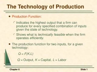
The Technology of Production • Production Function: • Indicates the highest output that a firm can produce for every specified combination of inputs given the state of technology. • Shows what is technically feasible when the firm operates efficiently. • The production function for two inputs, for a given technology: Q = F(K,L) Q = Output, K = Capital, L = Labor Chapter 6
Production Function for Food Labor Input 1 20 40 55 65 75 2 40 60 75 85 90 3 55 75 90 100 105 4 65 85 100 110 115 5 75 90 105 115 120 Capital Input 1 2 3 4 5 Chapter 6
Isoquants • Assumptions: Food producer has two inputs: Labor (L) & Capital (K) • Observations: 1) For any level of K, output increases with more L. 2) For any level of L, output increases with more K. 3) Various combinations of inputs produce the same output. • Isoquants: Curves showing all possible combinations of inputs that yield the same output Chapter 6
Production with Two Variable Inputs (L,K) Capital per year The Isoquant Map E 5 4 The isoquants are derived from the production function for output of of 55, 75, and 90. 3 A B C 2 Q3 = 90 D Q2 = 75 1 Q1 = 55 1 2 3 4 5 Labor per year Chapter 6
Isoquants The Short Run versus the Long Run • Short-run: • Period of time in which quantities of one or more production factors cannot be changed. These inputs are called fixed inputs. • Long-run • Amount of time needed to make all production inputs variable. Chapter 6
Production with One Variable Input (Labor) Amount Amount Total Average Marginal of Labor (L) of Capital (K) Output (Q) Product Product 0 10 0 --- --- 1 10 10 10 10 2 10 30 15 20 3 10 60 20 30 4 10 80 20 20 5 10 95 19 15 6 10 108 18 13 7 10 112 16 4 8 10 112 14 0 9 10 108 12 -4 10 10 100 10 -8 Chapter 6
Production with One Variable Input (Labor) • With additional workers, output (Q) increases, reaches a maximum, and then decreases. • The average product of labor (AP), or output per worker, increases and then decreases. Chapter 6
Production with One Variable Input (Labor) 3) The marginal product (MP) of labor or output of the additional worker increases rapidly initially and then decreases and becomes negative.. Chapter 6
D Total Product C A: slope of tangent = MP (20) B: slope of OB = AP (20) C: slope of OC= MP & AP B A Production with One Variable Input (Labor) Output per Month 112 60 Labor per Month 0 1 2 3 4 5 6 7 8 9 10 Chapter 6
Left of E: MP > AP & AP is increasing Right of E: MP < AP & AP is decreasing E: MP = AP & AP is at its maximum When MP=0, TP is at its maximum Marginal Product E Average Product Production with One Variable Input (Labor) Output per Month 30 20 10 Labor per Month 0 1 2 3 4 5 6 7 8 9 10 Chapter 6
Production with One Variable Input (Labor) The Law of Diminishing Marginal Returns • As the use of an input increases, a point will be reached at which the resulting additions to output decreases (i.e. MP declines). • When the labor input is small, MP increases due to specialization. • When the labor input is large, MP decreases due to inefficiencies. Chapter 6
Production with One Variable Input (Labor) The Law of Diminishing Marginal Returns • Can be used for long-run decisions to evaluate the trade-offs of different plant configurations • Assumes the quality of the variable input is constant, and a constant technology • Explains a declining MP, not necessarily a negative one Chapter 6
Labor productivity can increase if there are improvements in technology, even though any given production process exhibits diminishing returns to labor. C B O3 A O2 O1 The Effect of Technological Improvement Output per time period 100 50 Labor per time period 0 1 2 3 4 5 6 7 8 9 10 Chapter 6
Malthus and the Food Crisis • Malthus predicted mass hunger and starvation as diminishing returns limited agricultural output and the population continued to grow. Why did his prediction fail? • The data show that production increases have exceeded population growth. • Malthus did not take into consideration the potential impact of technology which has allowed the supply of food to grow faster than demand. Technology has created surpluses and driven the price down. • Question: If food surpluses exist, why is there hunger? Chapter 6
Production with One Variable Input (Labor) • Labor Productivity: AP = Total Output/Total Labor Input • Labor Productivity and the Standard of Living: Consumption can increase only if productivity increases. • Determinants of Productivity • Stock of capital • Technological change Chapter 6
Labor Productivity in Developed Countries United United France Germany Japan Kingdom States 1960-1973 4.75 4.04 8.30 2.89 2.36 1974-1986 2.10 1.85 2.50 1.69 0.71 1987-1997 1.48 2.00 1.94 1.02 1.09 Output per Employed Person (1997) $54,507 $55,644 $46,048 $42,630 $60,915 Annual Rate of Growth of Labor Productivity (%) Chapter 6
Production with One Variable Input (Labor) • Explanations for Productivity Growth Slowdown • Growth in the stock of capital is the primary determinant of the growth in productivity. Rate of capital accumulation in the US was slower than other developed countries, due to necessary rebuilding after WWII. • Depletion of natural resources • Environmental regulations Chapter 6
E A B C Q3 = 90 D Q2 = 75 Q1 = 55 Production with Two Variable Inputs: the Shape of Isoquants Capital per year 5 4 In the long run both labor and capital are variable and both experience diminishing returns. 3 2 1 1 2 3 4 5 Labor per year Chapter 6
Production with Two Variable Inputs Diminishing Marginal Rate of Substitution 1) Assume capital is 3 and labor increases from 0 to 1 to 2 to 3: note output increases at a decreasing rate illustrating diminishing returns from labor in the short-run and long-run. 2) Assume labor is 3 and capital increases from 0 to 1 to 2 to 3: note output increases at a decreasing rate (55, 20, 15) due to diminishing returns from capital. Chapter 6
Production with Two Variable Inputs • Substituting Among Inputs • The marginal rate of technical substitution equals: Chapter 6
2 1 1 1 Q3 =90 2/3 1 1/3 Q2 =75 1 Q1 =55 Marginal Rate of Technical Substitution Capital per year 5 Isoquants are downward sloping and convex like indifference curves. 4 3 2 1 1 2 3 4 5 Labor per month Chapter 6
Production with Two Variable Inputs MRTS and MP: the change in output from a change in labor equals: MRTS and MP: The change in output from a change in capital equals: Chapter 6
Production with Two Variable Inputs MRTS and MP: If output is constant and labor is increased, then: Chapter 6
A B C Q1 Q2 Q3 Isoquants When Inputs are Perfectly Substitutable Capital per month Labor per month Chapter 6
Q3 C Q2 B Q1 K1 A L1 Fixed-Proportions Production Function Capital per month Labor per month Chapter 6
Point A is more capital-intensive, and B is more labor-intensive. A 100 B 90 Output = 13,800 bushels per year Example: Isoquant Describing the Production of Wheat Capital (machine hour per year) 120 80 40 Labor (hours per year) 250 500 760 1000 Chapter 6
Example: Isoquant Describing the Production of Wheat 1) If the MRTS < 1, the cost of labor must be less than capital in order for the farmer to substitute labor for capital. 2) If labor is expensive, the farmer would use more capital (e.g. US). 3) If labor is inexpensive, the farmer would use more labor (e.g. India). Chapter 6
Increasing Returns to scale: The isoquants move closer together A 4 30 20 2 10 0 5 10 Firm Size and Output: Increasing Returns to Scale Capital (machine hours) Labor (hours) Chapter 6
A 6 30 4 20 2 10 0 5 10 15 Firm Size and Output: Constant Returns to Scale Constant Returns: Isoquants are equally spaced Capital (machine hours) Labor (hours) Chapter 6
A 8 30 2 20 10 0 5 20 Firm Size and Output: Decreasing Returns to Scale Capital (machine hours) Decreasing Returns: Isoquants get further apart Labor (hours) Chapter 6
The US Carpet Industry and Returns to Scale Carpet Shipments, 1996 (Millions of Dollars per Year) 1. Shaw Industries $3,202 6. World Carpets $475 2. Mohawk Industries 1,795 7. Burlington Industries 450 3. Beaulieu of America 1,006 8. Collins & Aikman 418 4. Interface Flooring 820 9. Masland Industries 380 5. Queen Carpet 775 10. Dixied Yarns 280 Chapter 6
Returns to Scale in the Carpet Industry • The carpet industry has grown from a small industry to a large industry with some very large firms. • Question: Can the growth be explained by the presence of economies to scale? • Are there economies of scale? • Costs (% of cost): Capital - 77%; Labor - 23% Chapter 6
Returns to Scale in the Carpet Industry • Large Manufacturers: Increased in machinery & labor; Doubling inputs has more than doubled output; Economies of scale exist for large producers • Small Manufacturers: Small increases in scale have little or no impact on output; Proportional increases in inputs increase output proportionally; Constant returns to scale for small producers Chapter 6