Download
1 / 34
340 likes | 428 Vues
Explore the intricacies of point processes on the line, nerve firing patterns, and building blocks of stochastic processes in R. Discover examples, properties, and applications of point processes through consistent sets of distributions and distributions. Dive into the analysis of point processes, autointensity, product densities, covariance, spectrums, and more. 8 Relevant

E N D
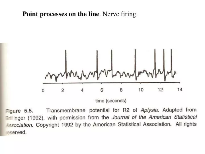
Stochastic point process. Building blocks Process on R {N(t)}, t in R, with consistent set of distributions Pr{N(I1)=k1 ,..., N(In)=kn } k1 ,...,kn integers 0 I's Borel sets of R. Consistentency example. If I1 , I2 disjoint Pr{N(I1)= k1 , N(I2)=k2 , N(I1 or I2)=k3 } =1 if k1 + k2 =k3 = 0 otherwise Guttorp book, Chapter 5
Points: ... -1 0 1 ... discontinuities of {N} N(t) = #{0 < j t} Simple: j k if j k points are isolated dN(t) = 0 or 1 Surprise. A simple point process is determined by its void probabilities Pr{N(I) = 0} I compact
Conditional intensity. Simple case History Ht = {j t} Pr{dN(t)=1 | Ht } = (t:)dt r.v. Has all the information Probability points in [0,T) are t1 ,...,tN Pr{dN(t1)=1,..., dN(tN)=1} = (t1)...(tN)exp{- (t)dt}dt1 ... dtN [1-(h)h][1-(2h)h] ... (t1)(t2) ...
Parameters. Suppose points are isolated dN(t) = 1 if point in (t,t+dt] = 0 otherwise 1. (Mean) rate/intensity. E{dN(t)} = pN(t)dt = Pr{dN(t) = 1} j g(j) = g(s)dN(s) E{j g(j)} = g(s)pN(s)ds Trend: pN(t) = exp{+t} Cycle: cos(t+)
Product density of order 2. Pr{dN(s)=1 and dN(t)=1} = E{dN(s)dN(t)} = [(s-t)pN(t) + pNN (s,t)]dsdt Factorial moment
Autointensity. Pr{dN(t)=1|dN(s)=1} = (pNN (s,t)/pN (s))dt s t = hNN(s,t)dt = pN (t)dt if increments uncorrelated
Covariance density/cumulant density of order 2. cov{dN(s),dN(t)} = qNN(s,t)dsdt st = [(s-t)pN(s)+qNN(s,t)]dsdt generally qNN(s,t) = pNN(s,t) - pN(s) pN(t) st
Identities. 1. j,k g(j ,k ) = g(s,t)dN(s)dN(t) Expected value. E{ g(s,t)dN(s)dN(t)} = g(s,t)[(s-t)pN(t)+pNN (s,t)]dsdt = g(t,t)pN(t)dt + g(s,t)pNN(s,t)dsdt
2. cov{ g(j ), g(k )} = cov{ g(s)dN(s), h(t)dN(t)} = g(s) h(t)[(s-t)pN(s)+qNN(s,t)]dsdt = g(t)h(t)pN(t)dt + g(s)h(t)qNN(s,t)dsdt
Product density of order k. t1,...,tk all distinct Prob{dN(t1)=1,...,dN(tk)=1} =E{dN(t1)...dN(tk)} = pN...N (t1,...,tk)dt1 ...dtk
Cumulant density of order k. t1,...,tk distinct cum{dN(t1),...,dN(tk)} = qN...N (t1 ,...,tk)dt1 ...dtk
Stationarity. Joint distributions, Pr{N(I1+t)=k1 ,..., N(In+t)=kn} k1 ,...,kn integers 0 do not depend on t for n=1,2,... Rate. E{dN(t)=pNdt Product density of order 2. Pr{dN(t+u)=1 and dN(t)=1} = [(u)pN + pNN (u)]dtdu
Autointensity. Pr{dN(t+u)=1|dN(t)=1} = (pNN (u)/pN)du u 0 = hN(u)du Covariance density. cov{dN(t+u),dN(t)} = [(u)pN + qNN (u)]dtdu
Mixing. cov{dN(t+u),dN(t)} small for large |u| |pNN(u) - pNpN| small for large |u| hNN(u) = pNN(u)/pN ~ pN for large |u| |qNN(u)|du < See preceding examples
Power spectral density. frequency-side, , vs. time-side, t /2 : frequency (cycles/unit time) Non-negative Unifies analyses of processes of widely varying types
Algebra/calculus of point processes. Consider process {j, j+u}. Stationary case dN(t) = dM(t) + dM(t+u) Taking "E", pNdt = pMdt+ pMdt pN = 2 pM
Association. Measuring? Due to chance? Are two processes associated? Eg. t.s. and p.p. How strongly? Can one predict one from the other? Some characteristics of dependence: E(XY) E(X) E(Y) E(Y|X) = g(X) X = g (), Y = h(), r.v. f (x,y) f (x) f(y) corr(X,Y) 0
Bivariate point process case. Two types of points (j ,k) Crossintensity. Prob{dN(t)=1|dM(s)=1} =(pMN(t,s)/pM(s))dt Cross-covariance density. cov{dM(s),dN(t)} = qMN(s,t)dsdt no ()
Frequency domain approach. Coherency, coherence Cross-spectrum. Coherency. R MN() = f MN()/{f MM() f NN()} complex-valued, 0 if denominator 0 Coherence |R MN()|2 = |f MN()| 2 /{f MM() f NN()| |R MN()|2 1, c.p. multiple R2
Proof. Filtering. M = {j } a(t-v)dM(v) = a(t-j ) Consider dO(t) = dN(t) - a(t-v)dM(v)dt, (stationary increments) where A() = exp{-iu}a(u)du fOO () is a minimum at A() = fNM()fMM()-1 Minimum: (1 - |RMN()|2 )fNN() 0 |R MN()|2 1
Proof. Coherence, measure of the linear time invariant association of the components of a stationary bivariate process.
Empirical examples. sea hare
Spectral representation approach. Filtering. dO(t)/dt = a(t-v)dM(v) = a(t-j ) = exp{it}dZM()
Partial coherency. Trivariate process {M,N,O} “Removes” the linear time invariant effects of O from M and N