Chapter 13 Random Utility Models
Chapter 13 Random Utility Models. This chapter covers choice models applicable where the consumer must pick one brand out of J brands. The sequence we will go through includes Terminology Aggregate Data and Weighted Least Squares Disaggregate Data and Maximum Likelihood

Chapter 13 Random Utility Models
E N D
Presentation Transcript
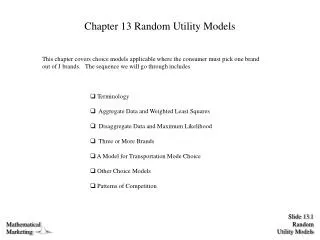
Chapter 13 Random Utility Models • This chapter covers choice models applicable where the consumer must pick one brand out of J brands. The sequence we will go through includes • Terminology • Aggregate Data and Weighted Least Squares • Disaggregate Data and Maximum Likelihood • Three or More Brands • A Model for Transportation Mode Choice • Other Choice Models • Patterns of Competition
Key Terminology • Dichotomous dependent variable • Polytomous dependent variable • Income type independent variable and the polytomous logit model. • Price type independent variable and the conditional logit model. • Aggregate data • Disaggregate dat
A Dichotomous Dependent Variable We define According to the regression model yi = 0 + xi1 + ei
How Do Choice Probabilities Fit In? From the definition of Expectation of a Discrete Variable
Two Requirements for a Probability Logical Consistency Sum Constraint
A Requirement for Regression Gauss-Markov Assumption V(e) = 2I Two possibilities exist Since E(ei) = 0 V(ei) = E[ei – E(ei)]2 by the Definition of E()
Heteroskedasticity Rears It’s Head Note that the subscript i appears on the right hand side!
Two Fixes Linear Probability Model Probit Model
The Expression for Not Buying where ui = 0 + xi1
The Logit Is a Special Case of Bell, Keeney and Little’s (1975) Market Share Theorem For J = 2 and the logit model, ai1 = and ai2 = 1
My Share of the Market Is My Share of the Attraction where a1 is a function of Marketing Variables brought to bear on behalf of brand 1
The Story of the Blue Bus and the Red Bus Imagine a market with two players: the Yellow Cab Company and the Blue Bus Company. These two companies split the market 50:50. Now a third competitor shows up: The Red Bus Company. What will the shares be of the three companies now?
Some Definitions ni = fi1 + fi2 pi1 = fi1 / ni
The Variance of the WLS Estimator So this allows us to test hypotheses of the form H0: a - c = 0
Multiple DF Tests Under WLS H0: A - c = 0
ML Estimation of the Logit Model Two equivalent ways of writing the likelihood We will use the left one, but isn't the right one clever?
Likelihood Derivations These first order conditions must be met:
Second Order ML Conditions When arranged in a matrix, the second order derivatives are called the Hessian. Minus the expectation of the Hessian is called the Information Matrix.
Three Choice Options pi1 + pi2 + pi3 = 1
Multinomial Logit Model the above model is a special case of the Fundamental Theorem of Marketing Share
Classic Example Ii Income of household i Cost (price) of alternative j for household i CAVi Cars per driver for household i BTRi Bus transfers required for member of household i to get to work via the bus
Other Choice Models Simple Effects Differential Effects Fully Extended MNL MCI
The Derivative Looks Like Here we have used the following two rules: dea/da = ea
The Elasticity for the Simple Effects MNL Model Putting the derivative back into the expression for the elasticity yields:

