Download
1 / 34
410 likes | 963 Vues
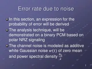
Error rate due to noise. In this section, an expression for the probability of error will be derived The analysis technique, will be demonstrated on a binary PCM based on polar NRZ signaling The channel noise is modeled as additive white Gaussian noise of zero mean and power spectral density .

E N D
Error rate due to noise In this section, an expression for the probability of error will be derived The analysis technique, will be demonstrated on a binary PCM based on polar NRZ signaling The channel noise is modeled as additive white Gaussian noise of zero mean and power spectral density
Bit error rate y(t) x(t) Y The receiver of the communication system can be modeled as shown below The signaling interval will be , where is the bit duration
Bit error rate The received signal can be given by It is assumed that the receiver has acquired knowledge of the starting and ending times of each transmitted pulse The receiver has a prior knowledge of the pulse shape, but not the pulse polarity
Receiver model The structure of the receiver used to perform this decision making process is shown below
Possible errors • When the receiver detects a bit there are two possible kinds of error • Symbol 1 is chosen when a 0 was actually transmitted; we refer to this error as an error of the first kind • Symbol 0 is chosen when a 1 was actually transmitted; we refer to this error as an error of the second kind
Average probability of error calculations To determine the average probability of error, each of the above two situations will be considered separately If symbol 0 was sent then, the received signal is
Average probability of error calculations The matched filter output will be given by The matched filter output represents a random variable Y
Average probability of error calculations This random variable is a Gaussian distributed variable with a mean of The variance of Y is The conditional probability density function the random variable Y, given that symbol 0 was sent, is therefore
Average probability of error calculations The probability density function is plotted as shown below To compute the conditional probability, , of error that symbol 0 was sent, we need to find the area between and
The integral Is known as the complementary error function which can be solved by numerical integration methods
By using the same procedure, if symbol 1 is transmitted, then the conditional probability density function of Y, given that symbol 1 was sent is given Which is plotted in the next slide
The probability of error that symbol 1 is sent and received bit is mistakenly read as 0 is given by
In order to find the value of which minimizes the average probability of error we need to derive with respect to and then equate to zero as From math's point of view (Leibniz’s rule)
If we apply the previous rule to , the n we may have the following equations By solving the previous equation we may have
From the previous equation, we may have the following expression for the optimum threshold point • If both symbols 0 and 1 occurs equally in the bit stream, then , then
A plot of the average probability of error as a function of the signal to noise energy is shown below
As it can be seen from the previous figure, the average probability of error decreases exponential as the signal to noise energy is increased For large values of the signal to noise energy the complementary error function can be approximated as
Example1 Solution
Example 3 solution Signaling with NRZ pulses represents an example of antipodal signaling, we can use
Example 3 solution Using the erfc(x) tablewe find With 3-dB power loss the power at the transmitting end of the cable would be twice the power at the receiving terminal, this means that