Download
1 / 39
510 likes | 1.35k Vues
SIGNAL TO NOISE RATIO CALCULATIONS FOR NOISE RADAR. Eric K. Walton The Ohio State Univ., ElectroScience Lab. Columbus, OH walton.1@osu.edu APS/URSI SYMPOSIUM, July 3-7, 2005 – Wash. D.C. URSI SESSION - RANDOM AND CHAOTIC RADAR. INTRODUCTION. BASIC NOISE RADAR CONCEPT.

E N D
SIGNAL TO NOISE RATIO CALCULATIONS FOR NOISE RADAR Eric K. Walton The Ohio State Univ., ElectroScience Lab. Columbus, OH walton.1@osu.edu APS/URSI SYMPOSIUM, July 3-7, 2005 – Wash. D.C. URSI SESSION - RANDOM AND CHAOTIC RADAR
INTRODUCTION BASIC NOISE RADAR CONCEPT A NOISE RADAR TRANSMITS (PSEUDO) RANDOM NOISE AND THEN PERFORMS A LARGE-SCALE CROSS CORRELATION TO DETECT THE REFLECTED SIGNAL.
PREVIOUS STUDIES:BUILDING PENETRATION Eric Walton; ESL
PREVIOUS STUDIES:BUILDING PENETRATION Concept for Dual Bistatic Building Penetration Radar Eric Walton; ESL
PREVIOUS STUDIES:BUILDING PENETRATION • SEQUENCE OF IMAGES SHOWING THE TRACKING OF A HUMAN AS HE WALKS FROM UPPER RIGHT TO LOWER LEFT. • THE HUMAN IS INSIDE A CONCRETE BLOCK BUILDING. • THE RADAR WAS APPROXIMATELY 50 FEET AWAY ON THE OUTSIDE. Eric Walton; ESL
pseudo- noise #1 clock antennas delay actually an array of antennas pseudo-noise #2 low pass filter output DIGITAL NOISE RADAR etc. Eric Walton; ESL PATENTED
IE: Target Specific Noise Radar Computer & digital I/O 100 MHz TRANSMIT WAVEFORM DATA LOAD (TX & RX) 64K x 9 FIFO Cypress CY7C4282 (100 MHz) MODULATED RF 100 MHz D/A BP Filt. TX 3.4 GHz LO ANTENNAS 3.4 GHz +/- 50 MHz Burr Brown DAC900 64K x 9 FIFO Cypress CY7C4282 (100 MHz) RIGHT LEFT 100 MHz D/A BP Filt. SW RX 100 MHZ RECEIVE WAVEFORM RECEIVED RF CLOCK 100 MHZ LOW PASS FILTER AUDIO BAND ANALOG DATA TO COMPUTER TARGET SPECIFIC DIGITAL NOISE RADAR PATENTED Eric Walton; ESL
PREVIOUS STUDIES(dual FIFO system) Teoman Ustun MS Thesis, Design and development of stepped frequency Continuous wave and fifo noise radar sensors For tracking moving ground vehicles OSU EE Dept, 2001.
PREVIOUS STUDIES(patented) ISSUED 3-8-05 6,864,834
PREVIOUS STUDIES 3.4 GHz Human Walking Toward the Radar Carrying C-Reflector Eric Walton; ESL
PREVIOUS STUDIES The raw data can be further processed using FFT processing. The final bandwidth then is the incremental bandwidth of the FFT. (sometimes called the bin bandwidth) In other words we get the signal processing gain of the FFT where a signal can be extracted from the noise. There are examples in some of my data where the signal can not be seen in the raw data but can be seen in the spectral (Doppler) plots. If we process 128 point FFT, for example, we get another factor of 128 signal processing gain.
PREVIOUS STUDIES DART DART (with screw) TENNIS BALL
SIGNAL TO NOISE CALCULATIONS Here is the model: Let us assume RCS of object: -40 DBSM (1 sq. cm.) Power transmitted: 0.25 watt Center Frequency: 10 GHz Antenna Power Gain: 5 wrt isotropic: (~7 dBi) Radar Range Equation : Eq. 1 Where Pr is the received reflected power and L is a set of loss factors lumped together (we use 0.5 here).
SIGNAL TO NOISE CALCULATIONS Next, we have signal power received due to thermal noise power at the receiver. Eq. 2where: k is Boltsman’s constant 1.38*10^-23, T= ambient temperature in deg. Kelvin (taken as 290 deg.) B = bandwidth in Hertz. (We use 300 MHz as the front end frequency bandwidth). This allows us to compute the pre-processing S/N ratio as Pr/Pn. Eq. 3. BUT: Don’t forget the LNA/mixer:
SIGNAL TO NOISE CALCULATIONS Then the signal processing power gain is based on the final audio filter BW. So:
SIGNAL TO NOISE CALCULATIONS • We wrote a MATLAB program to evaluate this equation. An example result is shown below for a specific set of conditions: • >> nradar • G (dB) = 6.9897 Ant. Gain • Pt = 0.25 Power trans. • R (m) = 30 Range in meters • RCS - DBSM = -40 Target RCS (DBSM) • Pr = 6.999e-016 Pow. Rec. (watts) • Pno = 1.2006e-012 Noise Pow. Rec. (watts) • SoNraw = 0.00058296 S/N power ratio - raw • Gsp = 60000 Signal processing gain • SoNfin = 34.9777 Final signal to noise power ratio • Prdbm = -121.5496 Rec. Power (dBm) • Pnodbm = -89.206 Rec. N. Power (dBm) • SoNfindb = 15.4379 S/N – post processing - dB • If we model it so that we get the post-processing S/N as a function of range, • we get figure 1.
SIGNAL TO NOISE CALCULATIONS Post processing S/N for -40 DBSM object (based on parameters from previous slide) Note that at +8 dB S/N, we can see this very small target out to 50 meters.
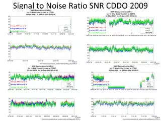
LETS TRY IT USING OUR EXAMPLE SOCCER BALL DATA • Soccer ball; 10 cm radius • σ = 4π r2 • 5 m (blue) • 7 m (green) • 9 m (red) • Measured Voltages (rel) • Sig= 15.5; 8.0; 16.2 • N = 1.2; 1.5; 2.1 • 20*log(S/N) = • 22 dB; 14 dB; 18 dB
TRY IT … MEASUREMENTS MEASUREMENTS
SIGNAL TO NOISE - DISPERSION NOTE THAT THE SPECTRAL DISPERSION OF THE SPHERE MAKES THE ABSOLUTE VALUE OF THE PEAK LOWER EVEN WHILE THE TOTAL ENERGY REMAINS HIGH. 600 dpi
REMEMBER THE BENEFITS OF DOPPLER PROCESSING DART DART (with screw) TENNIS BALL
DECORRELATON OF NARROW BAND CARRIERS 46 cm dia. sphere Interference
TRY IT … THEORETICAL RESULTS • Antenna gain = 5 dB • Ptx = 0.05 W • = 30/3.4 GHz = 8.8 cm • (metal sphere assumption for rubber soccer ball) • σ = π r^2 = 314 cm^2 = 25 DBSCM • T(noise) = 290 K • BW (RF) = 100 MHz • BW (final filter) = 10 kHz
SIMPLE S/N; BOTTOM LINE: • THE SIMPLE S/N CALCULATIONS : • Use the radar range equation to find received total reflected (noise) power • Does not account for non-optimum separation between signal and noise in the processor • such as a simple “peak threshold” • such as results from target/channel dispersion • Use “kTB” to compute noise • does not account for external interference (which may dominate because of the very wide bandwidths used in the noise radar) • does not account for the noise figure of the LNA/mixer combination • BUT THEY ARE STILL VERY USEFUL!
MORE DETAIL: Mathematical Description of the Noise Radar A noise signal can be written as (finite freq. band). This is a cosine Fourier Transform EXTRACTED FROM: “Signal to Noise Ratio Calculations and Measurements for the OSU Noise Radar” I. P. Theron, E. K. Walton, S. Gunawan and L. Cai, Technical Report 732168-1, The Ohio State Univ. ElectroScience Laboratory, Nov. 1996 The delayed signal is:
MORE DETAIL THE RECEIVED SIGNAL: The received signal consists of environmental noise and reflections from both the target of interest and clutter for an overall “target” transfer function of Next there is the propagation factor (delay and attenuation)
MORE DETAIL THE RECEIVED SIGNAL: The output of the mixer (mixing the received signal and the delayed transmitted signal) and remembering that the low pass filter will retain only the difference frequencies, we have This is the signal part of the S/N value.
MORE DETAIL … THE NOISE: So what is the “noise” part of the “signal – to - noise ratio”? • Output of low pass filter (without external noise) • External wide band noise sources • Lightning • Man-made unintentional signals • Jammers • External narrow band signal sources • Radio transmitters • Computer equipment IT IS NOT ALL “kTB” noise
MORE DETAIL … THE NOISE: • Noise from Low Pass Filter internal processes • Even in the absence of external noise, the LPF will contain DC and some low freq. noise as: Leaving out a number of steps, we eventually show that the output signal to noise ratio in the absence of environmental noise is: This is the best that we can hope for.
MORE DETAIL • EXTERNAL SOURCE OF WIDE BAND NOISE: • Assume an external signal with a flat spectrum but that is incoherent with the transmitted radar signal • Power computed as before ( ) • For large BW (noise) the total noise power is thus: • So the final S/N in this case is:
External source of narrow band signal: • Using similar logic, we can show that the average power at each frequency due to a narrow band source is based on the average power over the BW of the radar (IE: NsA2 ). • Thus we obtain the same total noise power as for the wide band external noise signal with a flat spectrum. • (We simply must compute the total external signal power in the BW of the radar.)
Final S/N including signal processing gain The signal power must be averaged in the t-domain and the noise power must be computed relative to the signal peak (IE: Lets assume a threshold target detection algorithm). If we plan on using a threshold level to determine the detection of a target, then we must consider the peak signal response to the peak noise response. (not the average noise power). We can thus compute the peak response of a random noise with a known power based on a useful number of statistical (sigma) widths. We usually find that the result yields a requirement of a factor of as much as 10 in the ratio of signal to noise to reliably “detect” a target. Of course, this depends on the desired ratio of false alarms to missed detections. (As does nearly all radar target detection processes.)
SUMMARY • WE HAVE SHOWN; • EXAMPLE NOISE RADAR DATA WITH NOISE • A SIMPLE WAY TO COMPUTE THE S/N • A SPECIFIC EXAMPLE COMPARISON BETWEEN MEASURED AND COMPUTED S/N • A MORE DETAILED APPROACH TO COMPUTATION OF S/N Dr. Eric Walton The Ohio State University ElectroScience Lab. Walton.1@osu.edu
NOISE RADAR PUBLICATIONS Publications: “Ultrawide-Band Noise Radar in the VHF/UHF Band,” (co-authors, I.P. Theron, S. Gunawan and L. Cai), IEEE Transactions Antennas Propagation, Volume 47 Number 6, pp. 1080-1084, Jun. 1999. “Compact Range Radar Cross Section Measurements Using a Noise Radar,” (co-authors, I.P. Theron and S. Gunawan), IEEE Trans. Antennas Propagation, Vol. 46, No. 9, pp. 1285-1288, Sep. 1998.
NOISE RADAR PUBLICATIONS Papers: “Development and Applications of a 16 Channel UHF/L-Band Noise Radar,” (co-author, S. Gunawan), Twentieth Annual Meeting and Symposium of the Antenna Measurement Techniques Association, pp. 210-213, Montreal, Canada, Oct. 26-30, 1998. “Signatures of Surrogate Mines using Noise Radar,” (co-author, L. Cai), AeroSense PIERS Meeting, Orlando, Florida, Apr. 13-17, 1998. “Future concepts for Ground Penetrating Noise Radar,” (invited paper) PIERS Workshop on Advances in Radar Methods, Joint Research Centre of the European Commission (Space Applications Institute), Baveno, Italy, Jul. 20-22, 1998. “Noise Radar A-P Mine Detection and Identification,” Demining MURI review, Night Vision Laboratory, Delphi, Maryland, Aug. 10-13, 1998. “Comparative Analysis of UWB Underground Data Collected Using Step-Frequency, Short pulses and Noise,” (co-author, S. Gunawan), Ultra-Wideband, Short Pulse Electromagnets 3, Proceedings of the Third International Conference on Ultra-Wideband, Short Pulse Electromagnetics, May 27-31, 1996, Albuquerque, New Mexico. (refereed; digest released as book for, Jan. 1997) “Moving Vehicle Range Profiles Measured Using a Noise Radar, “ (co-authors, I.P. Theron, S. Gunawan and L. Cai), 1997 IEEE AP-S Symposium and URSI Meeting, Montreal, Canada, Jul. 13-18, 1997. “Use of Fixed Range Noise Radar for Moving Vehicle Identification,” ARL 1997 Sensors and Electron Devices Symposium, College Park, MD, Jan. 14-15, 1997. “UWB Noise Radar Using a Variable Delay Line,” (co-authors, I. Theron and S. Gunawan), Nineteenth Annual Meeting and Symposium of the Antenna Measurement Techniques Association, Boston, Massachusetts, Nov. 17-21, 1997. “Comparative Analysis of UWB Underground Data Collected using Step-Frequency, Short Pulse and Noise Waveforms,” (co-author, S. Gunawan), AMEREM ‘96 International Conference on “The World of Electromagnetics” Albuquerque, New Mexico, May 27-31, 1996. “ISAR Imaging Using UWB Noise Radar,” (co-authors, V. Fillimon and S. Gunawan), Antenna Measurement Techniques Association Symposium, Seattle, Washington, Sep. 30-Oct. 3, 1996. “Comparison of Impulse and Noise-Based UWB Ground Penetrating Radars,” (co-author, F. Paynter), URSI Radio Science Meeting (Joint with AP-S), Seattle, WA, Jun. 19-24, 1994. “High Resolution Imaging of Radar Targets using Narrow Band Data,” (co-author, A. Moghaddar), Joint URSI Meeting and International IEEE/AP-S Symposium, London, Ontario, Jul. 1991. “Use of Stepped Delay Line Noise Radar for ISAR Imaging in the OSU Compact RCS Measurement Range,” (co-authors S. Gunawan), Joint Tech. Report 732168-2 and 727723-12, The Ohio State University ElectroScience Laboratory, Sep. 1997.