Download
1 / 102
1.02k likes | 1.09k Vues
This course delves into the concepts of signal and noise in fMRI data, covering topics such as signal size, SNR, noise properties, types of noise, Gaussian noise assumptions, variability in subject behavior, and methods for improving SNR. Emphasis is placed on understanding how to control and differentiate between signal and noise for accurate data interpretation in functional Magnetic Resonance Imaging (fMRI) studies.

E N D
Signal and NoiseII. Preprocessing BIAC Graduate fMRI Course October 19, 2005
What is signal? What is noise? • Signal, literally defined • Amount of current in receiver coil • How can we control the amount of received signal? • Scanner properties (e.g., field strength) • Experimental task timing • Subject compliance (through training) • Head motion (to some degree) • What can’t we control? • NOISE
Signal, noise, and the General Linear Model Amplitude (solve for) Measured Data Noise Design Model Cf. Boynton et al., 1996
E Signal Size in fMRI A 45 B 50 C 50 - 45 (50-45)/45 D
Voxel 1 790 830 870 Voxel 2 690 730 770 Voxel 3 770 810 850
Effects of SNR: Simulation Data • Hemodynamic response • Unit amplitude • Flat prestimulus baseline • Gaussian Noise • Temporally uncorrelated (white) • Noise assumed to be constant over epoch • SNR varied across simulations • Max: 2.0, Min: 0.125
SNR = 4.0 SNR = 2.0 SNR = .5 SNR = 1.0
What are typical SNRs for fMRI data? • Signal amplitude • MR units: 5-10 units (baseline: ~700) • Percent signal change: 0.5-2% • Noise amplitude • MR units: 10-50 • Percent signal change: 0.5-5% • SNR range • Total range: 0.1 to 4.0 • Typical: 0.2 – 0.5
II. Properties of Noise in fMRICan we assume Gaussian noise?
Types of Noise • Thermal noise • Responsible for variation in background • Eddy currents, scanner heating • Power fluctuations • Typically caused by scanner problems • Variation in subject cognition • Timing of processes • Head motion effects • Physiological changes • Differences across brain regions • Functional differences • Large vessel effects • Artifact-induced problems
Why is noise assumed to be Gaussian? • Central limit theorem • If X1 …Xn are a set of independent random variables, each with an arbitary probability distribution, then the sum of the set of variables (probability density function) will be distributed normally.
Variability in Subject Behavior: Issues • Cognitive processes are not static • May take time to engage • Often variable across trials • Subjects’ attention/arousal wax and wane • Subjects adopt different strategies • Feedback- or sequence-based • Problem-solving methods • Subjects engage in non-task cognition • Non-task periods do not have the absence of thinking What can we do about these problems?
A B C D E F Intersubject Variability A & B: Responses across subjects for 2 sessions C & D: Responses within single subjects across days E & F: Responses within single subjects within a session - Aguirre et al., 1998 Note: These data were collected using a periodic design that allowed timing of stimulus presentation. This served to exacerbate differences in HDR onset (e.g., some, but not all, subjects timed!).
Implications of Inter-Subject Variability • Use of individual subject’s hemodynamic responses • Corrects for differences in latency/shape • Suggests iterative HDR analysis • Initial analyses use canonical HDR • Functional ROIs drawn, interrogated for new HDR • Repeat until convergence • Requires appropriate statistical measures • Random effects analyses • Use statistical tests across subjects as dependent measure (rather than averaged data)
Spatial Variability? A B McGonigle et al., 2000
Spatial Distribution of Noise A: Anatomical Image B: Noise image C: Physiological noise D: Motion-related noise E: Phantom (all noise) F: Phantom (Physiological) - Kruger & Glover (2001)
Theoretical Effects of Field Strength • SNR = signal / noise • SNR increases linearly with field strength • Signal increases with square of field strength • Noise increases linearly with field strength • A 4.0T scanner should have 2.7x SNR of 1.5T scanner • T1 and T2* both change with field strength • T1 increases, reducing signal recovery • T2* decreases, increasing BOLD contrast
Measured Effects of Field Strength • SNR usually increases by less than theoretical prediction • Sub-linear increases in SNR; large vessel effects may be independent of field strength • Where tested, clear advantages of higher field have been demonstrated • But, physiological noise may counteract gains at high field ( > ~4.0T) • Spatial extent increases with field strength • Increased susceptibility artifacts
Trial Averaging • Static signal, variable noise • Assumes that the MR data recorded on each trial are composed of a signal + (random) noise • Effects of averaging • Signal is present on every trial, so it remains constant when averaged • Noise randomly varies across trials, so it decreases with averaging • Thus, SNR increases with averaging
Increasing Power increases Spatial Extent Subject 1 Subject 2 Trials Averaged 4 500 ms 500 ms 16 … 36 16-20 s 64 100 144
A B
Effects of Signal-Noise Ratio on extent of activation: Empirical Data Subject 1 Subject 2 Number of Significant Voxels VN = Vmax[1 - e(-0.016 * N)] Number of Trials Averaged
1000 Voxels, 100 Active Active Voxel Simulation Signal + Noise (SNR = 1.0) • Signal waveform taken from observed data. • Signal amplitude distribution: Gamma (observed). • Assumed Gaussian white noise. Noise
Effects of Signal-Noise Ratio on extent of activation:Simulation Data SNR = 1.00 SNR = 0.52 (Young) Number of Activated Voxels SNR = 0.35 (Old) SNR = 0.25 SNR = 0.15 SNR = 0.10 Number of Trials Averaged
Caveats • Signal averaging is based on assumptions • Data = signal + temporally invariant noise • Noise is uncorrelated over time • If assumptions are violated, then averaging ignores potentially valuable information • Amount of noise varies over time • Some noise is temporally correlated (physiology) • Nevertheless, averaging provides robust, reliable method for determining brain activity