Download
1 / 41
460 likes | 782 Vues
Signal and noise. Tiny signals in lots of noise. Rest. Pressing hands. % signal difference. Absolute difference. What’s the signal?. The signal we’re really measuring is tiny changes of current induced in our detector coils. What induces the current?

E N D
Tiny signals in lots of noise Rest Pressing hands % signal difference Absolute difference
What’s the signal? The signal we’re really measuring is tiny changes of current induced in our detector coils. What induces the current? What makes the signal in a voxel stronger (larger image intensity)? What is the “signal” we’re really interested in?
What’s the noise? • Thermal noise • System noise • Head motion, respiration, heart beat (physiological) noise • Hemodynamics variability • Neural variability • Behavioral/Cognitive variability Are 5&6 really noise?
Thermal noise Thermal motion of electrons, collisions, random exchange of energy, larger at higher temperatures… It is generally considered homogeneous and random and so can be reduced by averaging across multiple samples. It increases linearly with static field strength.
System noise Variability in the function of the imaging hardware across space and time. Static field inhomogeneities Scanner drift
Susceptibility artifacts Field inhomogeneities are particularly strong at tissue/air boundaries (sinuses). Increase with field strength. 1.5 T 4 T
Susceptibility correction You can measure the inhomogeneities in the magnetic field of your specific subject by “fieldmapping” them, and then correct the scan of the subject.
Head motion Moving the head during a scan causes two types of noise: Spatial changes throughout the scan.
Head motion Spatial changes can be estimated and fixed by locating brain edges and moving/rotating them appropriately. Now even done online by the scanner! Rather than post-hoc
Head motion • Image intensity artifacts in time (intensity “spikes”).
Head motion Intensity artifacts are more difficult to correct. Can either be “projected out”, interpolated over, or cut out. What happens when head motion and task are correlated?
Add motion parameters to model Add 6 predictors (3 translation and 3 rotation) to the model and hope they “soak” up the relevant variability. * + a1 a2 a3 a4 … error =
Or project/regress out Ensure zero correlation between the noise estimate (x) and the data (y). a = y*x y(after) = y(before) – a*x
Physiological noise There are non-neural mechanisms causing hemodynamic or inhomogeneity changes during a scan. Luckily they are periodical…
Respiration artifacts The lungs create a changing susceptibility artifact, similar to that seen below in the sinuses (stronger in larger fields). 1.5 T 4 T Only the lungs effect the signal throughout the brain…
Physiological noise Increases at higher static magnetic fields for the same reason the signal increases…
Temporal filtering High pass filter – lets the high frequencies pass, stops the low frequencies. Low pass filter – lets the low frequencies pass, stops the high frequencies. Band pass filter – lets a particular range of frequencies through (often by sequentially running a low high and low pass filter).
Hemodynamics variability Different subjects exhibit different HRFs
Hemodynamics variability HRFs vary across sessions Across brain areas?
Hemodynamics variability To address this we can estimate the subject’s HIRF in a separate run and use it to model the responses.
Neural variability The brain is never at “rest”, spontaneous neural activity fluctuations are as large as stimulus evoked responses.
Neural variability Some think the stimulus evoked responses “ride” on top of spontaneous cortical fluctuations, others think stimulus evoked responses replace spontaneous fluctuations. We typically get rid of them by averaging across multiple trials.
Behavioral/Cognitive variability The more complex an experiment, the more variable the behavioral responses: Subjects can choose different strategies. Changes in attention/arousal (caffeine). Response time distributions of two subjects performing a simple decision task.
Behavioral/Cognitive variability Again, variability is typically handled by averaging across trials. However, this variability also offers an opportunity: Does neural response amplitude predict reaction time or accuracy? fMRI response Reaction time
Intra-subject variability Finger tapping task
Intra-subject variability Generate random numbers
Improve SNR by averaging The main approach to canceling out noise is to average across multiple trials. This is a good approach for situations where noise is randomly distributed.
Improve SNR by averaging Estimating HRF using different trial numbers:
Improve SNR by averaging Estimating voxel significance using different trial numbers: Never compare statistics across conditions/groups. A difference in statistical significance does not equal a difference in signal strength!
Higher fields The signal is dependant on the magnetization of the hydrogen atoms, which increases with field strength (more atoms align with the static field). The gain in signal is quadratic. The increase in noise is linear. So the signal/noise ratio scales linearly with scanner strength.
Higher fields Stronger signal = finer spatial resolution (smaller voxels). But remember that we are limited to the resolution of the vasculature. There is already a lot of correlation among neighboring 3*3*3 mm voxels. Larger susceptibility artifacts. Shorter T2* Longer T1
Preprocessing Standard steps everyone does to reduce noise/variability:
Slice time correction Slices are acquired during different times within a TR:
Head motion correction Head motion artifacts are particularly evident at edges: The movement can generate a large change in image intensity, which can be correlated with the experiment design.
Head motion correction To avoid this sequential TR images are co-registered spatially and estimated head motion parameters are projected out of the data.
Distortion correction One can do a magnetic field mapping to determine inhomogeneities in the static magnetic field that cause geometric distortions
Temporal filtering Extract the part of the signal that’s related to your task. Or at least get rid of parts that aren’t (e.g. scanner drift). Squeeze hand for 20 seconds and then rest for 20 seconds.