Lake Clarity Model
120 likes | 255 Vues
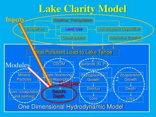
Lake Clarity Model. Inputs. Weather, Precipitation. Tributaries. Land Use. Atmospheric Deposition. Groundwater. Shoreline Erosion. Total Pollutant Load to Lake Tahoe. Modules. CDOM. Nutrients (N, P). Mineral Particles. Light Scattering and Absorption. Zooplankton Growth.

Lake Clarity Model
E N D
Presentation Transcript
Lake Clarity Model Inputs Weather, Precipitation Tributaries Land Use Atmospheric Deposition Groundwater Shoreline Erosion Total Pollutant Load to Lake Tahoe Modules CDOM Nutrients (N, P) Mineral Particles Light Scattering and Absorption Zooplankton Growth Phytoplankton Growth Output Detritus Death Secchi Depth Loss (coagulation and settling) Loss Loss One Dimensional Hydrodynamic Model
Input files to LCM LCM requires all weather forcing data, pollutant loads, lake and stream information, initial condition of lake, and parameters controlling the bio-chemical reactions.
Stream Inputs LSPC outputs : Flow volume and nutrients Particle counts : Rabidoux’s regression equation and LCPC flow Stream temperature : Artificial neural network and weather data
Stream Inputs Rabidoux (2005) developed statistically unbiased regression equations: P = 1 Q* + 0 Punbiased = exp(P) g(z) Where, P and Q are natural logarithms of particle flux (#/s) and stream flow (cfs), respectively; 0, and 1 are interception and slope of the log-log linear regression equation; g(z) is the Bradu and Mundlak (1970) correction factor for statistically unbiased estimation. Example
Storm water mean particle concentration (Source: Allan Heyvaert, DRI)
Multiplication Factor to Estimate Urban Particles Using Regression Equations Allan Heyvaert field data Average particle concentration for 0.49 - 16m = 3.4694 107 #/ml Rabidoux (2005) Average particle concentration for 0.49 - 16m = 1.0881 105 #/ml (Annual Average for the period 1994-2004) Multiplication factor for 0.5-16 m = (3.47 107)/ (1.09 105) = 318.9 Similarly, Multiplication factor for 16-63 m = (7.75 103)/ (3.54 102) = 21.9
Time-independent pollutant loadings to LCM Atmospheric load : LTADS report (CARB, 2006), UC Davis – TERC, DRI, UC Davis DELTA Group Groundwater load : USACOE [2003] Shoreline erosion : Adams and Minor [2002] estimates
Precipitation year selection (cont) Time dependent inputs Stream inputs Meteorological inputs Outflow inputs 1999 2000 2001 2002 … Precipitation year selection Time independent inputs • Atmospheric depositions • Groundwater loading • Shoreline erosion • Model parameters