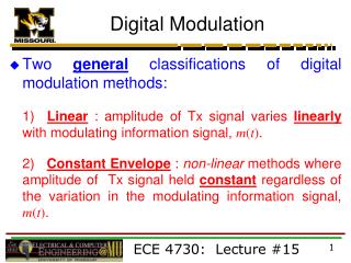
6.4 Digital Modulation

1. 6.4 Digital Modulation

2. 6.4 Digital Modulation • cost effective because of advances in digital technology • (VHDL, DSP, FPGA…) • digital vs analog • - digital has better noise immunity • - digital can be robust to channel impairments • - digital data can be multiplexed • - error control: detect & correct corrupt bits • - able to encrypt digital data • - flexible software modulation & demodulation • - digital requires complex signal conditioning • - digital is “all or nothing” 6.4.1 Factors in Digital Modulation 6.4.2 Bandwidth & Power Spectral Density (PSD) of Signals

3. 6.4.1 Factors in Digital Modulation

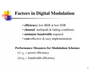
4. 6.4.1 Factors in Digital Modulation • modulating signal (message) represented as pulses • n bits represented by m finite states • n = log2m bitsper state • Significant Factors • efficiency: desire low BER at low SNR • channel: multipath & fading characteristics • minimize bandwidth required • cost and ease of implementation • Performance Measures for Modulation Schemes • (1)p = power efficiency • (2)B = bandwidth efficiency

5. (1) Power Efficiency, p • Ability to preserve signal fidelity at low power • increasing signal power  increases noise immunity • specifics depend on modulation technique • measures trade-off between fidelity & signal power p often expressed as ratio of Eb to N0at receiver input to achieve specified BER Eb / N0 =  to achieve BER <  Eb = bit energy N0= noise power spectral density

6. B=Rb/B 6.36 Fundamental Upper Bound on achievable Bit Rate per given Bandwidth (aka Shannon Bound) Bmax = C/B Bmax = log2 6.37 • C = maximum channel capacity (bps) • (2) Bandwidth Efficiency,B • Ability to accommodate data in limited bandwidth • increasing data rate  requires increased bandwidth • direct relationship to system capacity • measured in terms ofbit rate, Rb& RF bandwidth, B

7. B & p typically there is a tradeoff between • e.g • addition of error control codes increases p and decreases B • - increases bandwidth for given data rate • - reduces required received power for specified BER • use of M-ary keying increases B and decreases p • - decreases bandwidth for given data rate • - requires increased receive power for specified BER

8. Additional Factors in digital modulation • cost & complexity • cost vs performance improvement • complexity vs robustness • channel impairments (Rayleigh, Ricean fading) • multipath dispersion • interference from other users or random sources • detection sensitivity to timing jitter – time varying channel •  typically system is simulated & all factors are analyzed prior to • selection of methodsand specification of parameters

9. 6.4.2: Bandwidth & Power Spectral Density (PSD) of Signals

10. wT(t) wT(t) = 6.39 -T/2 T/2 PSD of w(t) is given by: Pw(f) = 6.38 • WT(f) is Fourier transform of wT(t) • bar denotes ensemble average of WT(f)2 6.4.2: Bandwidth & Power Spectral Density (PSD) of Signals assume w(t) is a randomsignal (measured in volts) let wT(t) be a truncated version of w(t)

11. real part imaginary part Fourier Transform of Real Even and Odd Signals for real signal x(t): X(f) = = • since cos(x) is an even function and sin(x) is an odd function: • X(-f) = X*(f) • Re[X(-f)] = Re[X(f)] • Im[X(-f)] = - Im[X(f)] • |X(-f)| = |X(f)| • X(-f) = -X(-f)

12. s(t) = Re(g(t)exp(j2fc)) 6.40 s(t) = bandpass (modulated) signal PSD of s(t) is related to PSD of g(t)by g(t) = complex envelope of baseband signal (magnitude & phase) • Pg(f) = PSD of g(t) • Ps(f) = PSD of s(t) Ps(f) = ¼[Pg(f-fc) + Pg(-f-fc)] 6.41 Bandpass vs Baseband Signals

13. i. absolute bandwidth = range of frequencies over which PSD  0 • for symbols represented as baseband pulses PSD has form of (sin f)2/f 2 - extends over infinite range of frequencies - absolute bandwidth =  Definitions of Bandwidth • ii. null-to-null bandwidth = bandwidth of main spectral lobe • simpler measure of bandwidth iii. ½ power bandwidth = frequency range between -3dB points iv. FCC definition: leaves exactly 0.5% of signal above upper band and below lower band (99% of signal power) v. outside a specified band, PSD < given level (e.g. 45dB, 60dB )

14. 6.5 Line Coding

15. 6.5 Line Coding • digital baseband signal often useline codes to provide spectral • characteristics of pulse train • i. RZ = pulse returns to 0 with every bit period • wider spectrum – easier to synchronize • ii. NRZ = pulse stays at constant level during bit period • narrower spectrum – harder to synchronize • iii. Manchester: 0-crossing guaranteed for each bit • Classification of line codes: • unipolar range = 0 .. V • bipolar range = -V.. +V • some line codes have dc components not used for circuits • that block dc signal (e.g. PSTN) • manchester has no dc component

16. (i) Unipolar NRZ weight ½ 0.5Tb V 0 1 0 1 0 … PSD t Rb 2Rb 3Rb f (ii) Bipolar RZ PSD 0.5Tb V -V 1 0 1 0 … t Tb 0.5Rb Rb 2Rb f Tb (iii) Manchester NRZ PSD V -V 1 0 1 0 … t 0.5Rb R 1.5Rb f Tb

17. 6.6 Pulse Shaping Techniques

18. 6.6 Pulse Shaping Techniques • Intersymbol Interference (ISI) • rectangular pulses passing through a bandlimited channel experience • delay spread from MPCs • ISI results when pulses smear – overlap with adjacent pulses • increasing channel bandwidth alleviates this, but often isn’t practical • e.g. mobile systems use techniques that reduce bandwidth and • suppress out-of-band radiation • - requires out-of-band radiation 40dB-80dB below • desired passband • Pulse Shaping: reduce spectral width (and ISI) of modulated data signal • pulse shaping done at basebandor IF • difficult to manipulate RF spectrum

19. 6.6.1 Nyquist Criteria for ISI Cancellation

20. Mathematical Statementof Nyquist Criteria Let heff(t) = system’s impulse response (transfer function) if n = 0 heff(nTs) = K 6.42 if n  0 heff(nTs) = 0 6.6.1 Nyquist Criteria for ISI Cancellation • Specifies system design criteria to nullify Effects of ISI • at receiver’sithsampling instant (recovering symbol i), the system • response for any symbolj  i is zero • system response includes transmitter, receiver, channel Ts= symbol period n is an integer K is non-zero constant Nyquist derived transfer function, Heff(f), which satisfied 6.42

21. heff(t) = (t)  p(t)  hc(t)  hr(t) 6.43 System transfer function satisfying Nyquist Criteria given as • pulse shape = p(t) • channel impulse response = hc(t) • receiver impulse response =hr(t) ( = convolution operation) • Two key considerations for selecting Heff(f)that satisfies 6.42 • (1) heff(t) should have fast decay & small magnitude near samples • at n  0 • (2) assume an ideal channel: hc(t) = (t), • requires an equalizer for FSF channels • reduces problem to designing approximate shaping filters at both • transmitter & receiver to produce desired Heff(f)

22. heff(t) = 6.44 xNYQ(t) 1 0.8 0.6 0.4 0.2 0 -0.2 -6T -4T -2T 0 2T 4T 6T heff(nTs) = 0 Consider Sinc Function: for n > 0 heff(nTs) = 0

23. Heff(f) = 6.45 Fourier Transform of sinc function yields • corresponds to “brick wall” filter with absolute bandwidth =fs/2 • fs=symbol rate (Hz) = 1/Ts (symbol period) • impulse response satisfies Nyquist condition for ISI cancellation • with minimal bandwidth • to eliminate ISI  model total system as filter with impulse • response of 6.44 including effects from • - transmitter filtering • - receiver filtering • - channel filtering

24. Heff(f) Frequency Response of Sinc Function f

25. practical issues: • (1) non-causal: heff(t)exists for t < 0  difficult to approximate • (2)sin t/tpulse has waveform slope = 1/t at each zero-crossing • waveform = 0 only at exact multiples of Ts • errors in sampling time of zero crossings (timing jitter) cause • sampling to occur when adjacent symbols to overlap • - results in significant ISI • - slope of 1/t2 or 1/t3 desirable - minimize ISI due to timing • jitter in adjacent samples

26. (2) Assume a filterexists with transfer function = rectangular filter • such that • f0  • f0= filter bandwidth • Ts = symbol period ISI solution based on sinc function and an even function in f • Nyquist also showed that if 2 conditions hold then frequency domain • convolution of filter & Z(f) satisfies zero ISI condition • (1) Assume functionZ(f)exists such that • Z(f) is an arbitrary even function: Z(f) = Z(-f) • Z(f) has zero magnitude outside passband of rectangular filter

27. Nyquist Criteria for zero-ISI is expressed mathematically as Heff(f) = 6.46 • for | f |  • f0  Z(f)=0 Impulse response expressed as heff(t) = 6.47

28. Nyquist Response Filter can eliminate ISI • entire communications link must have Nyquist Response • Transmitter mustfilter Baseband Signal to • constrain modulated BW to regulated values • minimize adjacent channel interference • Receiver mustfilter Incoming Signal to • remove strong interference • reject noise that is not the passband • therefore the following approach is taken • (i) split RC Filter between transmitter & receiver • (ii)assume channel response is flat (use adaptive equalizers, etc)

29. Assume channel distortion can be 100% neutralized by equalizer • equalizers transfer function =inverse of channel response • overall transfer function, Heff(f) can be approximated as • Heff(f) = HTX(f)HRX(f) HTX(f)= transmit filters transfer function HRX(f) = receive filters transfer function Effective end-end Heff(f) achieved using HTX(f) = HRX(f) = • provides matched filter response • minimizes bandwidth & ISI

30. 6.6.2 Raised Cosine (RC) Rolloff Filter

31. for 6.48 HRC(f) = for 0 for 6.6.2 Raised Cosine (RC) Rolloff Filter • popular pulse shaping filter with Nyquist Response (zero-ISI) • Transfer Function HRC(f)given as •  is the rolloff factor that determines transition bandwidth • 0    1 •  = 0  RC filter = rectangular filter with minimum bandwidth • Ts = 1/2Wmin (Wmin = minimum channel bandwidth) • = 1/Rb( Rb= bit rate)

32. cut off band range pass band range HRC(f) 1.0 0.5 0 transition band • RRC filter operating bands and response •  = 1 •  = 0.5 •  = 0

33. HNYQ(f) 1 scaling factor , 0 ≤  ≤ 1  = 0 Frequency Response for RRC filter for specific 

34. hRC(t) = 6.49 RC impulse response, hRC(t) obtained from IFT of HRC(f) • large hRC(t) decays faster at zero crossings • for t >>Ts rolloff  1/t3 • - less sensitive to timing jitter • - rapid rolloff allows temporal truncation with little penalty • temporal sidelobe levels decrease in adjacent symbol slots • however  occupiedbandwidth increases

35. 1/Ts HRC(f) 1.0 0.5 0 -Rs -¾Rs -½Rs 0 ½Rs ¾Rs Rs f -3Ts -2Ts -Ts 0 Ts 2Ts 3Ts RC filter impulse response and transfer function magnitude transfer function impulse response  = 1  = 0.5  = 0 • large : • increased bandwidth • faster decay  less sensitive to timing jitter • smaller temporal lobes

36. Baseband • Rs= feasible symbol rate through basebandRC filter • Ts = 1/Rs is symbol period • B = absolute filter bandwidth Rs = 6.50 ½ Rs ≤ B≤ Rsfor 0 ≤ ≤ 1 Passband For RF systems  passband bandwidth is doubled Rs = 6.51 Rs ≤ B≤ 2Rsfor 0 ≤ ≤ 1

37. Root Raised Cosine (RRC) • use identical filters at transmitter & receiver • filter transfer function = • matched filter realization provides optimum performance in flat • fading channel • filter can be implemented either at • baseband– before modulation • passband at transmitter output • typically – pulse shaping filters implemented using DSP at • baseband

38. hRC(t) -6Ts -5Ts-4Ts -3Ts -2Ts -Ts 0 Ts 2Ts 3Ts 4Ts 5Ts 6Ts 7Ts 8Ts 6Ts 6Ts • hRC(t) (6.49) is non-causal  must be truncated • for each symbol, pulse shaping filters typically implemented • for  6Tsabout t = 0 point • to reduce impact of truncation – modulator stores several symbols • at a time • group of symbols clocked out simultaneously – using lookup table

39. 1 0 1 0 Ts 2Ts 3Ts 4Ts 5Ts 6Ts 7Ts 8Ts 9Ts 10Ts • e.g. RC Filter with input binary pulses with = 0.5 • 3 bits (symbols) stored at a time  23 = 8 possible waveforms • if  6Ts represents time span for each symbol  time span of • discrete waveform = 14Ts • optimal bit decision points are zero-crossing points of other symbols • - don’t always coincide with peak values of waveform • - optimal decision points are 4Ts, 5Ts, and 6Ts • pulse is inherently time dispersive

40. p(t) 1.5 1.0 0.5 0 -0.5 -1.0 -1.5 -3 -2 -1 0 1 2 3 4 t/Tb e.g. pulse shaping comparison between RC and RRC • binary sequence 01100 • for binary ‘1’  multiply p(t) by ‘+’ symbol • for binary ‘0’  multiply p(t) by ‘-’ symbol -1 1 1 -1 -1 RRC shaping pulse p(t),α = 1.0 RC shaping pulsep(t),α = 0.5 RRC waveform occupies larger dynamic range than RC

41.  = 1.0  Bnull = 48.7 kHz Bnull = 32.9 kHz  = 0.35  Bnull = 24.35 kHz  = 0.0  e.g. assume Ts = 41.04us (Rs = 24.35k symbols/second) rectangular pulse, 1st zero crossing (null-to-null bandwidth) = 2/Ts = 48.7 kHz • RC filter • 1st zero crossing (null-to-null bandwidth) = • smaller  smaller Bnull, • bigger side lobes • more sensitive to timing jitter

42. 6.6.1.1 Practical Issues • 1. Finite Impulse Response (FIR) Filters • 2. Amplifiers: power efficiency vs linearity • 3. Symbol Timing Recovery • 1. FIR Filters (akadigital non-recursive linear phase filters) • can approximate perfect RRC filter to any accuracy for small  • as order of filter increases • - sharper transition bands occur • - longer processing time  more propagation delay

43. 2. Amplifiers • For RC filtersexact pulse shape must be preserved by carrier for • spectral efficiency • linear amplifiers preserve shape but are power inefficient • non-linear amplifiers are power efficient • - difficult to preserve pulse shape • - small distortions at baseband  can lead to large changes in • transmitted pulse • - can result in significant adjacent channel interference • For mobile communications – power efficiency is crucial ! • RC filters must use linear amplifiers with real-time feedback • to improve efficiency • *active research area

44. 3. Symbol Timing Recovery requires sampling of symbol • optimal zero-ISI sampling points = maximum eye opening • 3 methods: • (1) sendseparatetiming referenceas acontinuous tone at nTs • Ts = symbol period (e.g. seconds per symbol) • (2) send burst clock between message transmissions • (3) send timing information encoded into data (frequently used) • e.g.0-crossings in baseband bipolar data

45. 4. Symbol Timing Circuits needed for timing recovery because • large  is bandwidth inefficient • reducing results in sensitivity at zero-crossings however, • required bandwidth decreases towards minimum • noise in received signal causes imperfectzero-crossing • Practically, accept compromise between • quick symbol timing acquisition forrapid data decoding • long averaging time to minimize jitter

46. Ts/2 start timer sample zero crossings Ts • RRC filtered data with  = 1 timing of sample point is simplified • 0-crossings of filtered waveform occur at Ts/2before optimum zero • ISI detection points • start timer at 0-crossings sample data Ts/2 later • with strings of “000…” or “111…”  • - estimatecorrect sample times until next 0-crossing • - data scrambling or bit stuffing to increase frequency of 0-crossings

47. (1) Averaging over many 0-crossings can be used to • achieve accurate symbol timing on receiver with  < 1 • eliminate 0-mean noise • Feedback Timing Control Circuit • timing circuit has local clock, f(t) running at close to incoming Rs • monostable creates a pulse of duration Ts/2 at each 0-crossing • monostable & local clock are multiplied (mixed) • mixer output is integrated & filtered to produce smoothed DC voltage • - magnitude represents difference between incoming Rs & local clock • DC voltage is used to feed VCO to adjust local clock until it matches • incoming Rs • represents a compromise between • long averaging time to eliminate jitter • quick acquisition of symbol timing for rapid data decoding

48. a(t) b(t) c(t) e(t) f(t) 0-crossing detector mono-stable  VCO Ts/2 T’s a(t) b(t) f(t) c(t) e(t) increasing e(t)  increases frequency of f(t) decreasing e(t)  decreases frequency of f(t)

49. f0 = 1/2Ts t X2 2f0 = 1/Ts t 1/Ts f t • (2) square received filtered data stream • yields signal with strong discrete frequency component at symbol • timing frequency 2f0 = 1/Ts • extract signal with narrow band filter or PLL yields symbol • clock • - if  = 1 works well • - for small doesn’t yield discrete spectral line at 1/Ts

50. 6.6.3 Gaussian Pulse Shaping Filter