Lab. 3 Digital Modulation Digital modulation:
Lab. 3 Digital Modulation Digital modulation:. RF. {1,0,0,1,0,1,...}. Up- conversion. Transmit filter. Coder. DAC. symbol. noise. RF. Receive filter. Down- conversion. +. Channel. Baseband equivalent channel model. {1,0,0,1,0,1,...}. ADC. Processing. Detection. Decoder.

Lab. 3 Digital Modulation Digital modulation:
E N D
Presentation Transcript
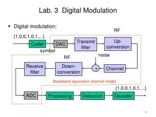
Lab. 3 Digital Modulation • Digital modulation: RF {1,0,0,1,0,1,...} Up- conversion Transmit filter Coder DAC symbol noise RF Receive filter Down- conversion + Channel Baseband equivalent channel model {1,0,0,1,0,1,...} ADC Processing Detection Decoder
Coder (symbol mapper): • Maps the input bits to a symbol (number). • Digital-to-analog converter (DAC) • Convert digital sequence to analogy waveform • Transmit filtering (pulse shaping): • Maps the symbol to an analog waveform. • Receiver filtering (matched filtering) • Match the transmit waveform (noise filtering) • Analog-to-digital conversion (ADC): • Convert analogy waveform to digital sequence (sampling) • Processing/detection • Process and detect the transmit symbol • Decoder: • Demaps the detected symbols to bits
Symbol mapping: • Transmit filtering: • Receive filtering: BPSK {1,0,0,1,0,1,...} Noise
Sampling: • Detection: • Demapping: {1,0,0,1,0,1,...}
Digital equivalent basebandchannel model: • Coder (symbol mapping): • PAM (1,3,5,7,..) • QAM (1/3/5/7,..+j 1/3/5/7) Noise Complex Channel h(n)
Practice 1: • Generate a 16-QAM mapper (Gray mapping). • Map a bit sequence with the mappers. (1110) (1010) (0010) (0110) (1111) (1011) (0011) (0111) (0001) (0101) (1101) (1001) (1100) (1000) (0000) (0100) * Note: there is no complex operations in C and you have to convert them into real operations
We first consider the baseband equivalent system. • Note that the operations of the digital systems can be exactly modeled. However, those of analog systems can only be approximately modeled. {1,0,0,1,0,1,...} Up- conversion Transmit filter Coder DAC symbol noise Receive filter Down- conversion + Channel Baseband equivalent channel model {1,0,0,1,0,1,...} ADC Processing Detection Decoder
Thus, we conduct simulations all on the digital domain. • This assumes that all the processing in analog domain is either perfect or can be absorbed into the channel and noise effects. noise {1,0,0,1,0,1,...} Digital Digital + Coder Channel symbol {1,0,0,1,0,1,...} Processing Detection Decoder
Detection: • Minimum error probability (maximize the posteriori probability) • For PAM: • For QAM: Decision boundary -1 3 -3 1
Practice 2 • Generate a 16-QAM sequence. • Add Gaussian noise to have a SNR of 10 dB. • Check if your generation is right. • Practice 3: • Conduct detection for the QAM symbols. • Calculate the probability of symbol error. *Signal power : 4(12+12)/16+8(12+32)/16+4(32+32)/16=10 10log10(10/2)=10 2=1 * You can write data to a file and use Matlab to plot or calculate. C: FILE *fp; fp = fopen("noise_r.dat","wb"); fwrite(nr,4,M,fp); fclose(fp); Matlab: fname=input('Input the file name?'); len=input('Input the data length?'); fid_1 = fopen(fname,'rb'); x = fread(fid_1,len,'float32'); fclose(fid_1); Length
Homework: • Simulate the symbol error rates (SERs) of the 16-QAM scheme with SNRs of 5dB, 10dB, 15dB, etc such that you can plot a SER curve. • Calculate the theoretical SERs and also plot a curve. • Put these two curves in the same figure to see if your simulation results are OK. Note: you may find that the result is different for different simulation.
rand() • Uniform random variable • between 0~RAND_MAX • #include <stdlib.h> • srand (time(NULL)); //Initialize random seed with system time • http://www.cplusplus.com/reference/cstdlib/rand/
Generate Gaussian Noise • Box-Muller method for generating Gaussian distributed random numbers • Generate z_1 and z_2 with U(-1,1), which can be done with z = 2y –1, y ~ U(0,1) • Discard (z_1, z_2) unless r^2 = z_1^2 + z_2^2 ≦ 1 • Consequently, we have