Lines and Arcs Segmentation
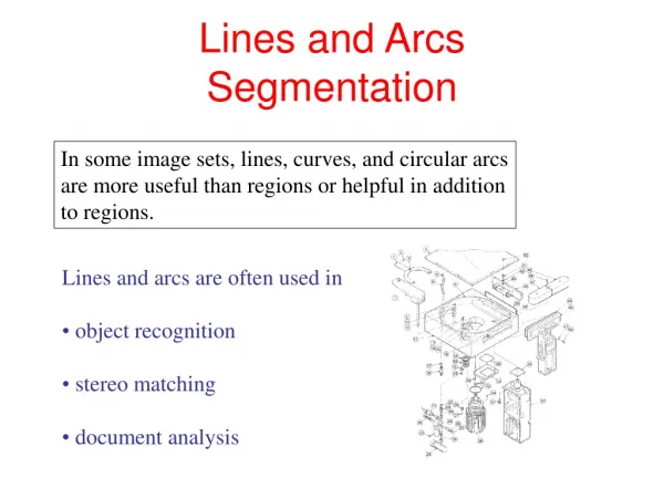
Lines and Arcs Segmentation. In some image sets, lines, curves, and circular arcs are more useful than regions or helpful in addition to regions. Lines and arcs are often used in object recognition stereo matching document analysis. Parameter Estimation Methods Hough Transform.

Lines and Arcs Segmentation
E N D
Presentation Transcript
Lines and ArcsSegmentation In some image sets, lines, curves, and circular arcs are more useful than regions or helpful in addition to regions. • Lines and arcs are often used in • object recognition • stereo matching • document analysis
Parameter Estimation MethodsHough Transform • The Hough transform is a method for detecting • lines or curves specified by a parametric function. • If the parameters are p1, p2, … pn, then the Hough • procedure uses an n-dimensional accumulator array • in which it accumulates votes for the correct parameters • of the lines or curves found on the image. accumulator image b m y = mx + b
Finding Straight Line Segments • y = mx + b is not suitable (why?) • The equation generally used is: d = r sin + c cos c d d is the distance from the line to origin is the angle the perpendicular makes with the column axis r
Procedure to Accumulate Lines • Set accumulator array A to all zero. • Set point list array PTLIST to all NIL. • For each pixel (R,C) in the image { • compute gradient magnitude GMAG • if GMAG > gradient_threshold { • compute quantized tangent angle THETAQ • compute quantized distance to origin DQ • increment A(DQ,THETAQ) • update PTLIST(DQ,THETAQ) } }
Example gray-tone image DQ THETAQ 0 0 0 100 100 0 0 0 100 100 0 0 0 100 100 100 100 100 100 100 100 100 100 100 100 - - 3 3 - - - 3 3 - 3 3 3 3 - 3 3 3 3 - - - - - - - - 0 0 - - - 0 0 - 90 90 40 20 - 90 90 90 40 - - - - - - Accumulator A PTLIST 360 . 6 3 0 - - - - - - - - - - - - - - - - - - - - - 4 - 1 - 2 - 5 - - - - - - - - - - - - - - - - - - - - - - - - - - - - * - * - * - * - - - - - - - 360 . 6 3 0 (3,1) (3,2) (4,1) (4,2) (4,3) distance angle 0 10 20 30 40 …90 (1,3)(1,4)(2,3)(2,4)
Chalmers University of Technology
Chalmers University of Technology
How do you extract the line segments from the accumulators? • pick the bin of A with highest value V • while V > value_threshold { • order the corresponding pointlist from PTLIST • merge in high gradient neighbors within 10 degrees • create line segment from final point list • zero out that bin of A • pick the bin of A with highest value V }
A Nice Hough VariantThe Burns Line Finder 45 2 3 3 4 2 +22.5 1 4 5 1 0 8 5 8 -22.5 6 7 6 7 1. Compute gradient magnitude and direction at each pixel. 2. For high gradient magnitude points, assign direction labels to two symbolic images for two different quantizations. 3. Find connected components of each symbolic image. • Each pixel belongs to 2 components, one for each symbolic image. • Each pixel votes for its longer component. • Each component receives a count of pixels who voted for it. • The components that receive majority support are selected.
2. Tracking Methods Mask-based Approach • Use masks to identify the following events: • 1. start of a new segment • 2. interior point continuing a segment • 3. end of a segment • 4. junction between multiple segments • 5. corner that breaks a segment into two junction corner
Edge Tracking Procedure for each edge pixel P { classify its pixel type using masks case 1. isolated point : ignore it 2. start point : make a new segment 3. interior point : add to current segment 4. end point : add to current segment and finish it 5. junction or corner : add to incoming segment finish incoming segment make new outgoing segment(s)
A Good Tracking Package: the ORT toolkit • Part of the C software available on the class web page • Updated versions are available • How does it work?
How ORT finds segments(Communicated by Ata Etemadi who designed it; this is really what he said.) • The algorithm is called Strider and is like a spider striding along pixel chains of an image. • The spider is looking for local symmetries. • When it is moving along a straight or curved segment with no interruptions, its legs are symmetric about its body. • When it encounters an obstacle (ie. a corner or junction) its legs are no longer symmetric. • If the obstacle is small (compared to the spider), it soon becomes symmetrical. • If the obstacle is large, it will take longer.
Strider • Strider tracks along a pixel chain, looking for junctions and corners. • It identifies them by a measure of assymmetry. • The accuracy depends on the length of the spider and the size of its stride. • The larger they are, the less sensitive it becomes.
Strider The measure of asymmetry is the angle between two line segments. L1: the line segment from pixel 1 of the spider to pixel N-2 of the spider L2: the line segment from pixel 1 of the spider to pixel N of the spider The angle must be <= arctan(2/length(L2)) angle 0 here Longer spiders allow less of an angle.
Strider • The parameters are the length of the spider and the number of pixels per step. • These parameters can be changed to allow for less sensitivity, so that we get longer line segments. • The algorithm has a final phase in which adjacent segments whose angle differs by less than a given angle are joined.
Advantages of Strider • works on pixel chains of arbitrary complexity • can be implemented in parallel • no assumptions and the effects of the parameters are well understood
Hough Transform for Finding Circles r = r0 + d sin c = c0 + d cos r, c, d are parameters Equations: Main idea: The gradient vector at an edge pixel points to the center of the circle. d *(r,c)
Why it works Filled Circle: Outer points of circle have gradient direction pointing to center. Circular Ring: Outer points gradient towards center. Inner points gradient away from center. The points in the away direction don’t accumulate in one bin!
Procedure to Accumulate Circles • Set accumulator array A to all zero. • Set point list array PTLIST to all NIL. • For each pixel (R,C) in the image { • For each possible value of D { • - compute gradient magnitude GMAG • - if GMAG > gradient_threshold { • . Compute THETA(R,C,D) • . R0 := R - D*cos(THETA) • . C0 := C - D* sin(THETA) • . increment A(R0,C0,D) • . update PTLIST(R0,C0,D) }}
Summary • The Hough transform and its variants can be used to find line segments or circles. • It has also been generalized to find other shapes • The original Hough method does not work well for line segments, but works very well for circles. • The Burns method improves the Hough for line segments and is easy to code. • The Srider algorithm in the ORT package gives excellent line and curve segments by tracking.