Download
1 / 26
270 likes | 577 Vues
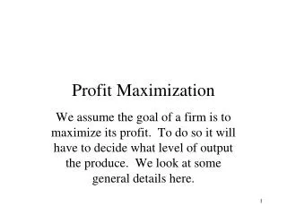
PROFIT MAXIMIZATION UNDER COMPETITIVE MARKET CONDITIONS. EA SESSION 8 18th July 2005 Prof. Samar K. Datta. Sub-topics to be covered. Perfectly Competitive Markets Profit Maximization Marginal Revenue, Marginal Cost, and Profit Maximization Choosing Output in the Short-Run

E N D
PROFIT MAXIMIZATION UNDER COMPETITIVE MARKET CONDITIONS EA SESSION 8 18th July 2005 Prof. Samar K. Datta
Sub-topics to be covered • Perfectly Competitive Markets • Profit Maximization • Marginal Revenue, Marginal Cost, and Profit Maximization • Choosing Output in the Short-Run • The Competitive Firm’s Short-Run Supply Curve • Short-Run Market Supply • Choosing Output in the Long-Run • The Industry’s Long-Run Supply Curve – Can it be less elastic?
MODELS OF MARKET STRUCTURE Market Structure Non-Atomistic Competition Atomistic Competition Oligopoly Duopoly Perfect Competition Monopolistic Competition Monopoly Conjectural Variation 0 Conjectural Variation = 0
Perfectly Competitive Markets • Characteristics of Perfectly Competitive Markets 1)Price taking 2) Product homogeneity 3) Free entry and exit
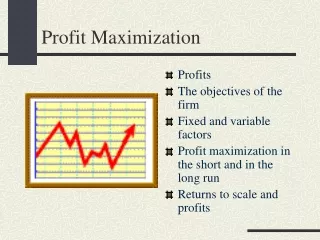
Cost, Revenue, Profit $ (per year) C(q) R(q) A B q0 q* 0 Output (units per year) Marginal Revenue, Marginal Cost,and Profit Maximization • Question • Why is profit reduced when producing more or less than q*?
$4 d $4 D Demand and Marginal Revenue Facedby a Competitive Firm Price $ per bushel Price $ per bushel Firm Industry Output (millions of bushels) Output (bushels) 100 200 100
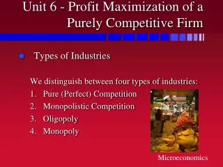
MC Lost profit for qq < q* Lost profit for q2 > q* A D AR=MR=P ATC C B AVC At q*: MR = MC and P > ATC q1 : MR > MC and q2: MC > MR and q0: MC = MR but MC falling q0 q1 q* q2 A Competitive FirmMaking a Positive Profit Price ($ per unit) 60 50 40 30 20 10 0 1 2 3 4 5 6 7 8 9 10 11 Output
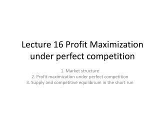
MC ATC B C D P = MR A At q*: MR = MC and P < ATC Losses = (P- AC) x q* or ABCD AVC F E q* A Competitive FirmIncurring Losses Price ($ per unit) Would this producer continue to produce with a loss? Output
Choosing Output in the Short Run • Summary of Production Decisions • Profit is maximized when MC = MR • If P > ATC the firm is making profits. • If AVC < P < ATC the firm should produce at a loss. • If P < AVC < ATC the firm should shut-down.
A Competitive Firm’sShort-Run Supply Curve S = MC above AVC Price ($ per unit) MC ATC P2 AVC P1 P = AVC Shut-down Output q1 q2
A Competitive Firm’sShort-Run Supply Curve • Observations: • Supply is upward sloping due to diminishing returns. • Higher price compensates the firm for higher cost of additional output and increases total profit because it applies to all units. • Firm’s response to an input price change • When the price of a firm’s input changes, the firm changes its output level, so that the marginal cost of production remains equal to the price.
The MC of producing a mix of petroleum products from crude oil increases sharply at several levels of output as the refinery shifts from one processing unit to another. SMC How much would be produced if P = $23? P = $24-$25? The Short-Run Productionof Petroleum Products Cost ($ per barrel) 27 26 25 24 Output (barrels/day) 23 8,000 9,000 10,000 11,000
S The short-run industry supply curve is the horizontal summation of the supply curves of the firms. MC1 MC2 MC3 P3 P2 P1 Industry Supply in the Short Run $ per unit Question: If increasing output raises input costs, what impact would it have on market supply? Quantity 0 2 4 5 7 8 10 15 21
The Short-Run Market Supply Curve • Perfectly inelastic (vertical) short-run supplyarises when the industry’s plant and equipment are so fully utilized that new plants must be built to achieve greater output. • Perfectly elastic (horizontal) short-run supply arises when marginal costs are constant.
The Short-Run Market Supply Curve • Producer Surplus in the Short Run • Firms earn a surplus on all but the last unit of output. • The producer surplus is the sum over all units produced of the difference between the market price of the good and the marginal cost of production.
At q* MC = MR. Between 0 and q , MR > MC for all units. Producer Surplus MC AVC B A P Alternatively, VC is the sum of MC or ODCq* . R is P x q*or OABq*. Producer surplus = R - VC or ABCD. D C q* Producer Surplus for a Firm Price ($ per unit of output) 0 Output
The Short-Run Market Supply Curve • Producer Surplus in the Short-Run • Observation • Short-run with positive fixed cost
In the long run, the plant size will be increased and output increased to q3. Long-run profit, EFGD > short run profit ABCD. LMC LAC SMC SAC D A E $40 P = MR C B G F $30 In the short run, the firm is faced with fixed inputs. P = $40 > ATC. Profit is equal to ABCD. q1 q2 q3 Output Choice in the Long Run Can this firm stay indefinitely at E? Price ($ per unit of output) Output
Choosing Output in the Long Run Long-Run Competitive Equilibrium • Entry and Exit • The long-run response to short-run profits is to increase output and profits. • Profits will attract other producers. • More producers increase industry supplywhich lowers the market price.
Profit attracts firms • Supply increases until profit = 0 S1 LMC P1 LAC S2 $30 P2 D Q1 Q2 Long-Run Competitive Equilibrium $ per unit of output $ per unit of output Firm Industry $40 q2 Output Output
Choosing Output in the Long Run • Long-Run Competitive Equilibrium 1) MC = MR 2) P = LAC • No incentive to leave or enter • Profit = 0 3) Equilibrium Market Price
Economic profits attract new firms. Supply increases to S2 and the market returns to long-run equilibrium. Q1 increase to Q2. Long-run supply = SL = LRAC. Change in output has no impact on input cost. S1 S2 MC AC C P2 P2 A B SL P1 P1 D1 D2 q1 q2 Q1 Q2 Long-Run Supply in aConstant-Cost Industry is a horizontal line $ per unit of output $ per unit of output 2 2 1 1 3 Sequence of events shown by numbers In both diagrams Output Output
Due to the increase in input prices, long-run equilibrium occurs at a higher price. S1 S2 LAC2 SMC2 SL SMC1 P2 LAC1 P2 P3 P3 B A P1 P1 D1 D1 q1 q2 Q1 Q2 Q3 Long-Run Supply in anIncreasing-Cost Industry is upward sloping $ per unit of output $ per unit of output 2 2 3 1 1 Sequence of events shown by numbers In both diagrams Output Output
Due to the decrease in input prices, long-run equilibrium occurs at a lower price. S1 S2 SMC1 LAC1 SMC2 P2 P2 LAC2 P1 A P1 B P3 P3 SL D1 D2 q1 q2 Q1 Q2 Q3 Long-Run Supply in anDecreasing-Cost Industry is downward sloping $ per unit of output $ per unit of output 2 2 1 1 3 Sequence of events shown by numbers In both diagrams Output Output
MC2 = MC1 + tax The firm will reduce output to the point at which the marginal cost plus the tax equals the price. MC1 An output tax raises the firm’s marginal cost by the amount of the tax. t P1 AVC2 AVC1 q2 q1 Effect of an Output Tax on a Competitive Firm’s Output (Is the drawing perfectly correct?) Price ($ per unit of output) Output
S2 = S1 + t S1 t P2 Tax shifts S1to S2and output falls to Q2. Price increases to P2. P1 D Q2 Q1 Effect of an OutputTax on Industry Output Price ($ per unit of output) Note how the burden of tax is generally borne by both parties Output