The Logistic Equation
The Logistic Equation. Robert M. Hayes 2003. Overview. Historical Context Summary of Relevant Models Logistic Difference Growth Model Linear Growth The Logistic Equation . Historical Context.

The Logistic Equation
E N D
Presentation Transcript
The Logistic Equation Robert M. Hayes 2003
Overview • Historical Context • Summary of Relevant Models • Logistic Difference Growth Model • Linear Growth • The Logistic Equation
Historical Context • The starting point for population growth models is The Principle of Population, published in 1798 by Thomas R. Malthus (1766-1834). In it he presented his theories of human population growth and relationships between over-population and misery. The model he used is now called the exponential model of population growth. • In 1846, Pierre Francois Verhulst, a Belgian scientist, proposed that population growth depends not only on the population size but also on the effect of a “carrying capacity” that would limit growth. His formula is now called the "logistic model" or the Verhulst model.
Recent Developments • Most recently, the logistic equation has been used as part of exploration of what is called "chaos theory". Most of this work was collected for the first time by Robert May in a classic article published in Nature in June of 1976. Robert May started his career as a physicist but then did his post-doctoral work in applied mathematics. He became very interested in the mathematical explanations of what enables competing species to coexist and then in the mathematics behind populations growth.
Summary of Relevant Models • Logistic growth models are derived from the exponential models by multiplying the respective factors r and (1+r) in the exponential models by (K – pt)/K. • Note that the two models for exponential growth are identical but the two for logistic growth are different. • The linear growth model is important both in itself and as a part of the logistic models.
Logistic Difference Growth Model • The logistic difference growth model will be considered in two contexts: • The Incremental Context, in which growth takes place at discrete points in time • The Continuous Context
The Incremental Context - I • Verhulst modified the exponential growth model to reflect the effect of a maximum for the size of the population. He denoted the carrying capacity as K and multiplied the ratio r in the difference exponential model by the factor (K - pt)/K to represent the effect of the maximum limit: (1) pt+1 = pt + ((K – pt)/K)*r*pt • Equivalently, (2) pt+1 – pt = ((K – pt)/K)*r*pt
The Incremental Context - II • Equation (2) will be called the logistic difference equation. The term "difference" emphasizes that the left hand side of the equation is the difference between successive values. • The following chart illustrates logistic difference growth, assuming a carrying capacity K = 1000, a growth rate r = 0.3, and a starting population p0 = 1. • At the start, with a small value of population, the factor (K – pt)/K will be very close to one, and the growth will be nearly exponential. • As the population value grows and gets closer to K, the factor will limit the population growth.
Illustrative Logistic Difference Growth • As this shows, the curve produced by the logistic difference equation is S-shaped. Initially there is an exponential growth phase, but as growth gets closer to the carrying capacity (more or less at time step 37 in this case), the growth slows down and the population asymptotically approaches capacity.
The Continuous Context • The differential counterpart to equation (6) is given by (3) dp = r*p(t)*(K – p(t))/K dt • There is a closed solution to this equation: (4) p(t) = K/(1 + ((K – p(0))/p(0))*e-r*t)
Linear Growth • Note that, qualitatively, there are three main sections of the logistic curve. The first has exponential growth and the third has asymptotic growth to the limit. But between those two is the third segment, in which the growth is virtually linear.
The Logistic Equation • Turning from the to the logistic population model to the "logistic equation": (7) pt+1 = ((K – pt)/K)*(1 + r)*pt = ((K – pt)/K)*s*pt, where s = 1 + r. • This equation exhibits fascinating behavior depending on the value of s = (1+r). We will illustrate the behavior with different values of s.
Some simple mathematical properties • First, though, there are two simple mathematical properties that will be of importance. To identify them, simplify the equation by letting pt = p and pt+1 = f(p) • The fixed points for f(p) occur whenf(p) = p, and that is either when p = 0 or when p = K – K/s = K*(s - 1)/s • The maximum value for pt occurs when the derivative of equation (10) is set to zero: (8) d f(p)/dp= s*(1 – 2*p/K) = 0, which can occur only if s = 0 (which is the minimum) or when p = K/2. At that value, pmax = s*K/4. • Since pmax K, s 4.
Decline to Zero (0 < s < 1) • When the value of s is between 0 and 1 (r 0) , the population will eventually decrease to zero. This is illustrated in the following graph, with K = 1000 and an initial population p0 = 500 individuals:
Normal Growth (1 < s < 3) - I • When the value of s is between 1 and 3, the population will increase towards a stable value. The following graph illustrates with three values of s (in each case, K = 1000 and p0 = 1.00):
Normal Growth (1 < s < 3) - II • Recall that the fixed points for f(p) occur at K*(1 – 1/s). For these three values of s, the fixed points therefore are at 200, 500, and 636. The three cases show very different speeds towards achieving their stable values. • One more thing to notice is that when the value of s is larger than 2.4, the equation shows an oscillation which is larger as it gets closer to 3.0, but in all cases the oscillation dies down and the population value settles down to its steady value.
Normal Growth (1 < s < 3) - III • One very interesting aspect of the logistic equation is that the long-term value of the population will be the same regardless of where it starts:
Multiple Stable Values (3 < s < 3.7) - I • When s reaches the value of 3, the population oscillates between two steady values, and at 3.4495 the population switches among four values! This effect continues, with oscillation among eight values when s = 3.56, sixteen values when s = 3.596, etc. • Note that for s > 3, there is truly a spectacular rate of growth—more than tripling in each time period. It is therefore not surprising that there should be a rebound as the population bounces against its upper limit and then recovers rapidly only to rebound again. • The following charts show three graphs of this behavior:
At s = 3.00, the oscillation is among two values and at 3.55, among four values.
Chaos (3.7 < s < 4) • When s reaches a value of 3.7, the population jumps in what appears to be a random, unpredictable way, and it behaves so until s reaches a value 4.0. While this behavior looks random, it really isn't. • This phenomenon has been called "chaos“, first used to describe this phenomenon by James A. Yorke and Tien Yien Li in their classic paper "Period Three Implies Chaos" [American Mathematical Monthly 82, no. 10, pp. 985-992, 1975] • The following graph uses a value of r = 3.75.
Solutions to the Logistic Equation • There are only three values of s for which there are closed form solutions to the logistic equation. To simplify, let K = 1, so that f(p) = s*p*(1 – p) • For s = 4, f(pn) = (1 – cos(2n*g))/2, where g = cos-1(1 – 2 p0) • For s = 2, f(pn) = (1 – exp(2n*g), where exp(x) = ex and g = log(1 – 2*p0) • For s = – 2, f(pn) = 1/2 – cos( + (-2)n*g), where g = cos-1(1 – 2 p0)