The Heat Equation
Time Dependent Problem. The Heat Equation. time step. Example:. Time Dependent Problem. The Heat Equation. Weak Formulation ( variational formulation). Fix a time t. Multiply equation (1) by and then integrate over the domain. Green’s theorem gives.

The Heat Equation
E N D
Presentation Transcript
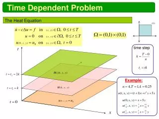
Time Dependent Problem The Heat Equation time step Example:
Time Dependent Problem The Heat Equation Weak Formulation ( variational formulation) Fix a time t Multiply equation (1) by and then integrate over the domain Green’s theorem gives
Variational Formulation BVP Spatial Discretization
Spatial Discretization Crank-Nicolson Method
Time Discretization case case
Time Discretization case case case case case case
Time Discretization Solve the linear system of equations to find Solve the linear system of equations to find Solve the linear system of equations to find Solve the linear system of equations to find
Computer Implementation function [u1]=HeatSolver2D(p,e,t) k = 0.001; % time step T = 0.07; % final time n = T/k; np = size(p,2); % number of nodes x = p(1,:)'; y = p(2,:)'; % node coordinates u1 = sparse(np,n); % set zero IC ix=find(sqrt(p(1,:).^2+p(2,:).^2)<0.4); u1(ix,1)=ones(size(ix)); M = MassMatrix(p,t); %primary mass matrix A = StiffMatrix(p,t); %primary stiff matrix [A,M] = boundary(A,M,p,t,e); % M,A after imbosing boundary bound = unique([e(1,:) e(2,:)]); % boundary nodes inter = setdiff([1:np],bound); % interior nodes bold = Vec_b(0,p,e,t,bound,inter); for l = 2:n % time loop time = l*k; bnew = Vec_b(time,p,e,t,bound,inter); LHS = (M + 0.5*k*A); % Crank-Nicholson rhs = (M - 0.5*k*A)*u1(inter,l-1) + 0.5*k*(bnew + bold); bold = bnew; u1(inter,l) = LHS\rhs; end % draw.m %To speed up the plotting, we interpolate to a rectangular grid. x=linspace(-1,1,31);y=x; [unused,tn,a2,a3]=tri2grid(p,t,u1(:,1),x,y); % Make the animation newplot; nframes = size(u1,2); Mv = moviein(nframes); umax=max(max(u1)); umin=min(min(u1)); for j=1:nframes,... u=tri2grid(p,t,u1(:,j),tn,a2,a3);i=find(isnan(u));u(i)=zeros(size(i));... surf(x,y,u);caxis([uminumax]);colormap(cool),... axis([-1 1 -1 1 0 1]);... %contourf(x,y,u);colormap(cool) Mv(:,j) = getframe;... pause(0.01) end download all files
Computer Implementation function M = MassMatrix(p,t) np = size(p,2); nt = size(t,2); M = sparse(np,np); for K = 1:nt loc2glb = t(1:3,K); % local-to-global map x = p(1,loc2glb); % node x-coordinates y = p(2,loc2glb); % node y- area=polyarea(x,y); MK = [2 1 1; 1 2 1; 1 1 2]/12*area; % element mass matrix M(loc2glb,loc2glb) = M(loc2glb,loc2glb)+ MK; end function [A,M] = boundary(A,M,p,t,e); np = size(p,2); % total number of nodes bound = unique([e(1,:) e(2,:)]); % boundary nodes inter = setdiff([1:np],bound); % interior nodes A = A(inter,inter); % modify stiffness matrix M = M(inter,inter); % Mass matrix matrix function [area,b,c] = Gradients(x,y) area=polyarea(x,y); b=[y(2)-y(3); y(3)-y(1); y(1)-y(2)]/2/area; c=[x(3)-x(2); x(1)-x(3); x(2)-x(1)]/2/area; function b = Vec_b(time,p,e,t,bound,inter); f = inline('time.*sin(x).*cos(y)','time','x','y'); np = size(p,2); nt = size(t,2); b = zeros(np,1); for K = 1:nt loc2glb = t(1:3,K); x = p(1,loc2glb); y = p(2,loc2glb); area = polyarea(x,y); bK = [f(time,x(1),y(1)); f(time,x(2),y(2)); f(time,x(3),y(3))]/3*area; % element load vector b(loc2glb) = b(loc2glb)+ bK; % add element loads to b end b = b(inter); % modify load vector function A = StiffMatrix(p,t) np = size(p,2); nt = size(t,2); A = sparse(np,np); for K = 1:nt loc2glb = t(1:3,K); % local-to-global map x = p(1,loc2glb); % node x-coordinates y = p(2,loc2glb); % node y- [area,b,c] = Gradients(x,y); AK = (b*b'+c*c')*area; % element stiff mat A(loc2glb,loc2glb) = A(loc2glb,loc2glb)+ AK; end
T=0 One time step After 10 time steps Steady state solution
Heat Equation spatial semi-discretization equation Fully discrete Equation
1 given the primary mass matrix M Consider the heat equation 5/24 1/24 1/24 1/24 0 0 1/24 1/24 1/24 5/24 0 1/24 1/24 1/24 1/24 0 1/24 0 1/12 1/48 0 0 0 1/48 1/24 1/24 1/48 1/8 1/48 0 0 0 0 1/24 0 1/48 1/12 1/48 0 0 0 1/24 0 0 1/48 1/12 1/48 0 1/24 1/24 0 0 0 1/48 1/8 1/48 1/24 0 1/48 0 0 0 1/48 1/12 and the primary stiffness matrix A 4 0 -1 -1 0 0 -1 -1 0 4 0 -1 -1 -1 -1 0 -1 0 1 0 0 0 0 0 -1 -1 0 2 0 0 0 0 0 -1 0 0 1 0 0 0 0 -1 0 0 0 1 0 0 -1 -1 0 0 0 0 2 0 -1 0 0 0 0 0 0 1 For the numerical solution, we use the following triangulation a) Write down the semidiscrete equation. b) Apply the forward Euler method with k = 1/3 and then write down the fully discrete equation. c) Use part (b) to estimate u(1, 3/2, 3/2)