Download
1 / 37
370 likes | 627 Vues
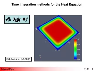
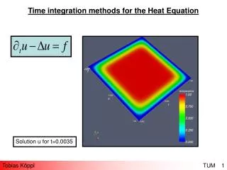
Time integration methods for the Heat Equation. Solution u for t=0.0035. Tobias Köppl TUM. 1. Agenda:. 1. Time integration methods. 1.1. Implicit and explicit Onestep Methods.

E N D
Time integration methods for the Heat Equation Solution u for t=0.0035 Tobias Köppl TUM 1
Agenda: 1. Time integration methods 1.1. Implicit and explicit Onestep Methods 1.2. Convergence theory for Onestep Methods 2. The Heat Equation 2.1. Discretization of the Laplacian operator 2.2. Application of Time integration methods 2.3. Courant-Friedrichs-Levy condition 3. Outlook 4. Literature Tobias Köppl TUM 2
Notation: : field of real numbers : vector space of d dimensional vectors with components, which are in : is a differentiable function, which maps from the intervall into and whose derivative function is continous partial derivative of y with respect to t Laplacian operator of y Machine accuracy with Tobias Köppl TUM 3
1. Time integration methods 1.1. Implicit and explicit Onestep Methods Goal: Find numerical approximations of functions which are solutions of an ODE with an initial value: (IVP) Tobias Köppl TUM 4
Example (IVP): 1. Time integration methods 1.1. Implicit and explicit Onestep Methods Dahlquist‘s Testequation Tobias Köppl TUM 5
Construction of a time integration method by discrete timepoints: Divide the continous intervall t on Grid Stepsize of grid : Approximation of the solution at the gridpoints for all 1. Time integration methods 1.1. Implicit and explicit Onestep Methods by a gridfunction Tobias Köppl TUM 6
Additionaly: Computation of the gridfunction by recursion, should be possible. Such algorithms are called Onestep Methods. Reason: For the computation of only from the timepoint Further possibility: Multistep Methods. before is needed. See literature for more information f.e. [DB II] Chapter 7 or [QSS] Chapter 11 1. Time integration methods 1.1. Implicit and explicit Onestep Methods Tobias Köppl TUM 7
explicit Euler Method: implicit Euler Method: 1. Time integration methods 1.1. Implicit and explicit Onestep Methods Two popular Onestep Methods are the explicit and the implicit Euler Method: Tobias Köppl TUM 8
Construction of: Compute the tangent vector t in Compute the intersection point between: and First component of this intersection point is the next value of the gridfunction 1. Time integration methods 1.1. Implicit and explicit Onestep Methods Geometry of the explicit Euler Method: t t Source: [DB II] The explicit Euler Method is creating a path (Euler path). Tobias Köppl TUM 9
Definition (local discretization error): The local discretization error of a gridfunction for a grid on the intervall is defined as: is the solution of the IVP: on 1. Time integration methods 1.2. Convergence theory for Onestep Methods Issue: Under which conditions does a Onestep Method converge towards the exact solution of an ODE with an initial value? Tobias Köppl TUM 10
Definition: A Onestep Method is called constistent, if: for Theorem: The explicit and the implicit Euler Method are consistent. 1. Time integration methods 1.2. Convergence theory for Onestep Methods Proof: See f. e. [DB II] Chapter 4. Tobias Köppl TUM 11
Definition (global discretization error): The global discretization error is the maximum error between the computed approximations and the corresponding values of the exact solution for 1. Time integration methods 1.2. Convergence theory for Onestep Methods Defintion (convergence): A Onestep Method is called convergent towards the exact solution of an IVP, if: Tobias Köppl TUM 12
1. Time integration methods 1.2. Convergence theory for Onestep-Methods Comparison of local and global Discretization error: Source: [Bun] Tobias Köppl TUM 13
Defintion (stability): A numerical algorithm is called (numerically) stable, if for all permitted input data perturbed in the size of computational accuracy ( ) acceptable results are produced under the influence of rounding and method errors. Maintheorem of Numerics: A Onestep Method is convergent, if and only if it is consistent. 1. Time integration methods 1.2. Convergence theory for Onestep-Methods Tobias Köppl TUM 14
Theorem: The implicit Euler Method is stable for any stepsize The explicit Euler Method is only stable for small Example: If , the explicit Euler Method is a stable integrator for Dahlquist‘s testequation. 1. Time integration methods 1.2. Convergence theory for Onestep-Methods Remark: Stability of a Onestep Method is an essential condition for getting qualitatively correct solutions, when using practical stepsizes. See numerical experiment. Proof: See f. e. [Jun] Chapter 4. Tobias Köppl TUM 15
Goal: Find a numerical approximation of the two dimensional Laplacian operator in order to solve the Poisson equation: 2. The Heat Equation 2.1. Discretization of the Laplacian operator (PE) Tobias Köppl TUM 16
Discretization Method: Finite Differences Main idea: Replace differential operators by difference operators Further discretization methods: Finite Volumes or Finite Elements See literature for more information f.e. [QSS] or [Wa] 2. The Heat Equation 2.1. Discretization of the Laplacian operator Tobias Köppl TUM 17
Discretization of Discretizationpoints: and Uniform grid with grid parameter h 2. The Heat Equation 2.1. Discretization of the Laplacian operator Tobias Köppl TUM 18
2. The Heat Equation 2.1. Discretization of the Laplacian operator Source: [Hu] Tobias Köppl TUM 19
Discretization of the two dimensional Laplacian operator: Discretization error: 2. The Heat Equation 2.1. Discretization of the Laplacian operator is an interior point of the unit square expand and in a Taylor series around expand and in a Taylor series around Tobias Köppl TUM 20
In order to get a numerical solution of the (PE) we have to solve the following System of linear equations: Matrix- Vectornotation: 2. The Heat Equation 2.1. Discretization of the Laplacian operator (SLSE) Tobias Köppl TUM 21
Use fast iterative solvers like Jacobi Method or Gauß Seidel Method for the solution of (SLSE) 2. The Heat Equation 2.1. Discretization of the Laplacian operator Structure of the Matrix A: A ist a sparse Matrix See f.e. [El] Source: [Hu] Tobias Köppl TUM 22
2. The Heat Equation 2.1. Discretization of the Laplacian operator Example: Solution: See numerical example Tobias Köppl TUM 23
2. The Heat Equation 2.2. Application of Time integration methods Goal: Find numerical approximations of functions which are solutions of the homogenous Heat Equation: Tobias Köppl TUM 24
h h 2. The Heat Equation 2.2. Application of Time integration methods Solution of the Heat Equation depends on time and space. Discretization of time and space is necessary Both time and space can be discretized by an uniform grid Source: [SK] Tobias Köppl TUM 25
Discretization of Uniform grid (2D) with grid parameter h Uniform grid (1D) with stepsize k and n timepoints Discretization of 2. The Heat Equation 2.2. Application of Time integration methods Discretizationpoints: and timepoints: Tobias Köppl TUM 26
Construct a local IVP for every 2. The Heat Equation 2.2. Application of Time integration methods (IVP(ij)) Tobias Köppl TUM 27
Solve IVP(ij) with the implicit Euler Method: Use the discretization of the two dimensional Laplacian Operator: 2. The Heat Equation 2.2. Application of Time integration methods Tobias Köppl TUM 28
Use again fast iterative solvers like Jacobi Method or Gauß Seidel Method for the solution of (SLSE II) 2. The Heat Equation 2.2. Application of Time integration methods We have to solve the following system of linear equations for every timestep: (SLSE II) Tobias Köppl TUM 29
Numerical Example: (Cooling of a heated plate) 2. The Heat Equation 2.2. Application of Time integration methods Tobias Köppl TUM 30
(IVP(ij)) can be solved by the explicit Euler Method, too. Chapter 1.2.: explicit Euler Method is only stable for a small stepsize k Maintheorem of Numerics: Stability is an essential condition for getting qualitatively correct solutions, when using practical stepsizes. 2. The Heat Equation 2.3. Courant-Friedrichs-Levy condition Tobias Köppl TUM 31
h h 2. The Heat Equation 2.3. Courant-Friedrichs-Levy condition Theorem (CFL condition): The explicit Euler Method is a stable solver for the Heat Equation if: Proof:See [CFL] Source: [SK] Tobias Köppl TUM 32
Numerical Example: (Cooling of a heated plate, solved with the explicit Euler Method and a discretization which is not conform with the CFL condition) 2. The Heat Equation 2.3. Courant-Friedrichs-Levy condition Tobias Köppl TUM 33
x(t) x(t) t Adaptive discretization algorithms, with a good error measurement are required An uniform discretization of the time axis, would lead to a Onestep Method with slow convergence 3. Outlook Let x(t) be the solution of an (IVP): Source: [DH I] Tobias Köppl TUM 34
3. Outlook Further topics: Optimization of the algorithms, solving the sparse linear equation systems, with respect to storage and number of floating point operations Traversing a certain grid efficiently (peano curves) Preconditioning of the Matrix representing the mentioned SLSE Tobias Köppl TUM 35
4. Literature: [DH I]: Numerische Mathematik I, Deuflhard/Hohmann, 2002, 3. edition [DB II]: Numerische Mathematik II, Deuflhard/Bornemann, 2002, 2. edition [Jun]: Lecture on Numerische Mathematik, Junge, 2007 [SK]: Numerische Mathematik, Schwarz/Köckler, 2006, 6. edition [QSS]: Numerische Mathematik 2, Quateroni/Sacco/Saleri, 2002, 2. edition [Wa]: Lecture on Finite Elements, Wall, 2007, 2. edition [Hu]: Numerics for computer sience students, Huckle/Schneider, 2002, 3. edition [Bun]: Lecture on numerical programming, Bungartz, 2007 [El]: Finite Elements and Fast Iterative Solvers, Elman/Silvester/Wathen, 2005, 2. ed. [Fo I]: Analysis I, Forster, 1976, 6. edition [Fo II]: Analysis II, Forster, 1976, 6. edition [Fei]: Introduction into the theory of partial differential equations, 2000 [CFL]: Über die partiellen Differentialgleichungen der mathematischen Physik, Courant, Friedrichs, Levy, 1928 Tobias Köppl TUM 36
Thank you for your attention!!! Tobias Köppl TUM 37