Diagnostics II
Diagnostics II. Mark Rodwell. Meteorological Training Course Predictability, Diagnostics and Extended-Range Forecasting. ECMWF. 10 May 2012. Talk Outline. Barotropic Rossby Waves Rossby Wave ‘Source’ Diabatic Processes Flow-Dependent Error Precipitation. Barotropic Rossby Waves.

Diagnostics II
E N D
Presentation Transcript
Diagnostics II Mark Rodwell Meteorological Training Course Predictability, Diagnostics and Extended-Range Forecasting ECMWF 10 May 2012
Talk Outline • Barotropic Rossby Waves • Rossby Wave ‘Source’ • Diabatic Processes • Flow-Dependent Error • Precipitation
Observations. 300–100 hPa vΨ, vχ & RWS Group Velocity Phase Velocity 10-10s-2 Contour 8ms-1 24 May 25 May 26 May 27 May 2008
The Vorticity Equation z y x is the unit “vertical” vector and is the horizontal curl operator Curl of the 3D momentum equation in absolute frame of reference: Shallow atmosphere approximation & assuming non-divergent, horizontal, barotropic, frictionless flow: Motivation (2D flow) :
Barotropic Rossby Wave Solutions Where Non-divergent barotropic vorticity equation Seeking wave-like solutions … We obtain the ‘dispersion relation’ Where Rossby waves get advected downstream and propagate upstream The larger the spatial scale of the wave, the faster the upstream propagation For stationary waves Mid-latitude stationary zonal wavenumbers
Observations. 300–100 hPa vΨ, vχ & RWS Group Speed Phase Speed 10-10s-2 Contour 8ms-1 24 May 25 May 26 May 27 May 10ms-1 agrees well with theory 2008
Stationary Rossby Waves 10-11 s-2 Sig. 10% Non sig. Upstream Propagation Downstream Advection Advection by Anomalous Rotational Wind Advection of Anomalous Vorticity 40-year mean response to change in aerosol climatology deduced using seasonal-mean data. Results are very similar when daily data are used. Anomalies integrated 100-300 hPa.
Upper Troposphere Divergent Wind Anomaly New minus Old aerosol. Anomaly is integrated between 100 and 300 hPa
The Rossby Wave Source When divergent winds are not neglected in the vorticity equation Application to barotropic models: Sardeshmukh and Hoskins (1988) For use in complex GCMs, it is found here to be useful to vertically integrate this equation between 100 and 300 hPa
Balance in Vorticity Equation: New Aerosol-Old 10-11 s-2 Sig. 10% Wave Initiators Non sig. Upstream Propagation Downstream Advection Rossby Wave Source The Rossby Wave Source is indeed seen as the tropically induced source of the extratropical stationary Rossby wave response Advection by Anomalous Rotational Wind Advection of Anomalous Vorticity 40-year mean JJA response to change in aerosol climatology deduced using seasonal-mean data. Results are very similar when daily data are used. Anomalies integrated 100-300 hPa.
Aerosol impact summary: RWS, vχ, Ψ (& mean ζ) 10-11 s-2 40-year mean JJA response to change in aerosol climatology deduced using seasonal-mean data. Anomalies integrated 100-300 hPa. Rossby wave paths agree beautifully with those predicted by Hoskins and Ambrizzi (1995)
Precipitation, v925 and Z500. New Aerosol-Old mm day-1. 10% Sig. 40-year mean JJA response to change in aerosol climatology deduced using seasonal-mean data.
RWS, vχ and Meridional wind anomalies Look at developments like this from PV perspective. • Classic example that led to a forecast ‘bust’ over Europe a few days later • What is the diabatic forcing? • How well does the (first guess) forecast represent this forcing? • What are the implications of observation rejection? 30 May 5 June Incoming Rossby wave 6 June RWS shade interval 10-10 s-2. Meridional wind contour interval 8 ms-1. 100-300 hPa integrals
European forecast ‘busts’ ACC of Z500 over Europe
Trends in bust frequency A bust is defined as when the day-6 Z500 forecast has European RMSE>60m and ACC<40%
Composite conditions during a bust Z500 ‘Blocking High’ Mediterranean Depression Using all 584 ERA Interim busts that occurred between the dates 1 January 1989 - 24 June 2012.
Initial conditions preceding a bust Using all 584 ERA Interim busts that occurred between the dates 1 January 1989 - 24 June 2012.
Z500 spread and error for trough/CAPE situation 84 trough/CAPE situations Background Using dates 10 November 2010 - 20 March 2012.Accounting for annual cycle in background errors and spread
Potential Vorticity budget @ 330K for trough/CAPE By modifying the stratification, diabatic processes appear to oppose the advection term and slow the propagation of the wave Contours show composite PV anomaly Shading shows PV budget terms
Analysis of winter storm “Lothar” TROPOPAUSE FOLDING ASSOCIATED WITH KURT AND ISENTROPIC DOWN-GLIDING(?) CYCLONE “KURT” LOW-LEVEL CYCLONE “LOTHAR” 18Z, 25 DEC1999 PV=2 SURFACE V850 Wernli et al. (2002) Fig. 7a
Analysis of winter storm “Lothar” CYCLONE “KURT” TROPOPAUSE FOLD NOW ALSO ASSOCIATED WITH LOTHAR LOW-LEVEL CYCLONE “LOTHAR” 0Z, 26 DEC1999 PV=2 SURFACE V850 Wernli et al. (2002) Fig. 7b
Analysis of winter storm “Lothar” CYCLONE “KURT” LOW-LEVEL CYCLONE “LOTHAR” UPPER AND LOWER PV ANOMALIES NEARLY JOIN INTENSE WINDS KILL 50 6Z, 26 DEC1999 PV=2 SURFACE V850 Wernli et al. (2002) Fig. 7c
Verification as a tool for decision-making • Application to Precipitation
A probabilistic score for precipitation (RPS) Categories defined by climatology with p2=2p3 Brier Score 2-category proper score Ranked Probability Score 3-category proper score tD/L tL/H RPS rewards system for forecasting each category with the ‘true’ probability
RPS trends in ensemble forecast Lead-time to RPS/RPSc=1 Extra-tropics Lead-time (days) Date Improving trend but revised uncertainty estimates (as well as flow dependence) make this noisy. Can we assess the (deterministic) model component separately?
RPS applied to deterministic forecasts Mean RPS 1 June - 31 August 2010 (24-hr accumulations) ‘Hedging’ of deterministic forecast is rewarded (as with Brier Score). Different approach needed
A deterministic score for precipitation (SEEPS) Categories defined by climatology with p2=2p3 Peirce Skill Score (PSS) 2-category equitable score SEEPS 3-category equitable score tD/L tL/H SEEPS (Stable Equitable Error in Probability Space) rewards system for forecasting each category with the observed frequency
Error features penalised by SEEPS: 16/12/2008 Over-prediction of drizzle to north. Over-prediction of alpine convection. Failure to predict convection along southern coast of France
Error features penalised by SEEPS: 23/08/2008 Failure to predict heavy precipitation ahead of Low over northern Europe, too much frontal precipitation to the south
Category Frequencies andSEEPS Contributions Heavy precipitation important later in forecast Under-prediction of dry weather Over-prediction of light precipitation Drizzle from the start hinders score Good frequency of heavy precipitation
SEEPS score trends Lead-time to SEEPS=0.6 (relative to ERA Interim) Extra-tropics Lead-time difference (days) Date Trends can be clearly identified. Control shows immediate benefits of each resolution change. High Resolution system tends to advance after subsequent physics updates
SEEPS model comparison 24-hour precipitation at day 4 (global average) ECMWF generally in lead
SEEPS as measure of ensemble spread Observation representativity and SEEPS’ sensitivity to climatology are issues to investigate
Combined Prediction System (CPS): Methodology Each ensemble member (orange squares) has unit weight. Find the weight to give to the high-resolution forecast (the size of the yellow rectangle) by optimising a probabilistic score (e.g. BSS for precipitation > 1mm)
The weight to give the high-resolution system 2001-2005 At short lead-times, high-resolution system is very valuable. At longer lead-times weight →1
Combined system is more skilful 2001-2005 Important: Results are cross-validated so no artificial inflation of skill
Summary • Barotropic Rossby Waves • Natural modes of extratropical variability • Rossby Wave ‘Source’ • Diagnosing links to the tropics • Diabatic Processes • Forecast busts • Spread–Error relationship • Flow-Dependent Error • Verification as a diagnostic tool • Ensemble system using proper RPS score • Deterministic forecast using equitable SEEPS score • Combined forecast system

