Modeling Virtual Stability in Complex Systems: Insights from Population Simulations
This research explores the concepts of stability and transitions in complex adaptive systems through population simulations. The assumption that such systems predominantly reside in stable states is discussed alongside the Principle of Selective Retention, which posits that stable configurations are maintained while unstable ones are eliminated. The study delves into discrete state space models, revealing how adaptive control mechanisms influence system trajectories. Notably, the implications for environmental and cognitive systems are examined, highlighting critical thresholds and the challenges of reversing catastrophic transitions.

Modeling Virtual Stability in Complex Systems: Insights from Population Simulations
E N D
Presentation Transcript
Modeling Virtual Stability With a Population Simulation Burton Voorhees & Joseph Senez Center for Science Athabasca University Supported by NSERC Discovery Grant OGP 0024817, NSERC Undergraduate Student Research Assistantships, and grants from the Athabasca University Research Fund
Contributors: Todd Keeler Rhyan Arthur National Science and Engineering Research Council of Canada Undergraduate Summer Research Assistants Martin Connors Professor of Physics, Center for Science, Athabasca University
The Assumption of Stability The standard assumption: Complex systems will be found in states that are stable, or at least metastable, with only occasional brief periods of transition between such states. The Principle of Selective Retention: “Stable configurations are retained, unstable ones are eliminated.” Heylighen
Discrete State Space Models Discrete models of complex systems generally assume that the system state space is partitioned into basins of attraction, determined by system dynamics. Each basin represents a coarse-grained state of relative stability. State space trajectories remain in a given basin unless driven to another by system dynamics; or until perturbed sufficiently by noise.
Discrete State Space Models Robert May outlined the intuition behind this idea, arguing that only small regions in a system parameter space can provide long term stability. Note, however, that the system state space is not the same as its parameter space, but state space dynamics can lead to dynamical changes in parameter values.
Discrete State Space Models Stable states are determined by a fitness landscape: the instantaneous system state remains near a fitness peak. Applied specifically to models of evolution, a species is characterized by a set of phenotypic parameters and parameter values are expected to cluster in relatively small regions falling within constraints imposed by selective fitness barriers defining this peak.
Course Graining State space trajectories are represented as a discrete time series of transitions on a finite set of states. In this course-grain version of the continuous representation each basin of attraction corresponds to a distinct state in the discrete model.
Control Course-grained trajectories of complex adaptive systems are not random. They represent adaptive responses to environmental contingencies, or (in systems with a cognitive component) goal directed action sequences. In either case, the course-grained system trajectory is determined by adaptive control mechanisms.
Control and Transition Control studies are especially important when human value judgments are associated to the possible coarse-grained states of a complex system. Both theoretical models and empirically studied exemplary cases show that catastrophic jumps between attractor basins do occur, and that such jumps may be exceptionally difficult to reverse.
Control and Transition Typically, a coarse-grained state appears relatively unchanged over time, while system parameter values change slowly in a way that drives the system trajectory toward an attractor basin boundary, or weakens the strength of the attractor, leaving the system vulnerable to small fluctuations that move it to a new attractor basin. A sudden jump of coarse-grained state occurs and, due to hysteresis effects, returning system parameters to earlier values does not reverse the jump.
Example: Ecology “The pristine state of most shallow lakes is probably one of clear water and a rich submerged vegetation. Nutrient loading has changed this situation in many cases. Remarkably, water clarity seems to be hardly affected by increased nutrient concentrations until a critical threshold is passed, at which the lake shifts abruptly from clear to turbid. With this increase in turbidity, submerged plants largely disappear. …Reduction of nutrient concentration is often insufficient to restore the vegetated clear state. Indeed, the restoration of clear water happens at substantially lower nutrient levels than those at which the collapse of the vegetation occurred.” M. Scheffer, S. Carpenter, J.A. Foley, C. Folke, & B. Walker (2001) Catastrophic shifts in ecosystems. Nature413 591-596
Psychology/Neurophysiology “The core idea is to interpret mental representations as more or less stable attractors… and states encoding the sensory information about the stimuli as initial conditions….” Empirical results from experiments on bistable perception suggest that transitions between the two possible perspectives on the Necker cube illusion transit through an unstable “saddle” between two relatively stable attractors. In this case, it is a matter of the projection of a three dimensional object from a two dimensional image. The unstable state is the objective perception of this two dimensional image, without the projection of a third dimension. Anybody who makes the attempt will find that it requires effort to maintain this perception—we have learned to automatically see in three dimensions. J. Kornmeier, M. Bach, & H. Atmanspacher (2004) Correlates of perceptive instabilities in event-related potentials. International Journal of Bifurcation and Chaos14(2) 727-736.
Examples such as these illustrate the centrality of stability and instability for every area of complex systems theorizing.
Ashby’s Law of Requisite Variety In order to maintain systemic integrity in a fluctuating environment the variety of responses available to a system must be at least as great as the variety in the spectrum of environmental perturbations. There is an additional factor not taken into account in this criteria.
The Importance of Instability In terms of management and control, it is not only a matter of maintaining a system in a desired state, but of managing state transitions. It is not only a matter of maintaining sufficient variety in a set of possible responses, but also of being able to switch between responses in a timely manner.
The Importance of Instability This implies the existence of a trade-off between stability and flexibility. It is easy to change an unstable state, difficult to change a stable one: if a possible behavioral response state is stable, change consumes time and energy; if not stable, it is easy to change, but energy is required to maintain it.
The Importance of Instability If behavioral responses at the physiological, neural, and habitual levels are relatively stable attractors, then avoidance of commitment to an immediate response is like remaining on an unstable boundary between possible attracting behaviors. Maintaining such a state requires effort and so exacts a cost. What is purchased by the energy expended is increased behavioral flexibility in the face of uncertainty.
Example: Standing The standing posture is learned in early childhood and automated as an unstable state, maintained by a process of proprioceptive feedback and small muscular adjustments. The resulting flexibility shows up in the ease of walking. If standing were stable, the stability would act as an attractive force maintaining the state. Every step would require effort to overcome the stability and would feel like walking uphill. As it is, taking a step is a controlled fall.
Virtual stability • A state in which a system employs self-monitoring and adaptive control in order to maintain itself in a configuration that would otherwise be unstable. • A degree of instability is maintained, at a certain cost, in order be able to quickly adapt/move to a desired state.
Virtual Stability • Not the same as stability or metastability • Stability: There is a single global attractor, or the system is deterministic and once an attractor basin is entered system trajectories remain there. If there is noise, the system is stable against “small” perturbations. • Metastability: A system has multiple attractor basins with fractal boundaries containing chaotic saddles. Basin boundary dimensions are close to the dimension of the full state space. Even a small amount of noise can produce transitions between attractor basins. • Virtual Stability: Through processes of self-monitoring and adaptive control a system maintains itself on a boundary between two or more attractor basins.
Condition for Virtual Stability Meta-level control functions direct the expenditure of energy to maintain an unstable trajectory, or an unstable state. At a minimum, this requires that a system have the capacity to monitor its momentary state and produce adaptive responses at a frequency high enough that only small (i.e., inexpensive) corrective actions are required.
The Popsim program • The advantages/disadvantages of virtual stability are explored by comparing a population of three types of individuals (A, B or C) in a varying sequences of three different environments (A, B, or N). • Stability and instability are modeled with probability. Populations A and B are stable, with only a small chance of transition from A to B or vice versa. Members of population C are virtually stable--they can easily make transitions to both A and B. When members of population C are acting as A, they are said to be in the state AC, when they are acting as B they are said to be in the state BC. • The program seeks conditions and sequences of environments that will favor the stable A and B populations OR the virtually stable C population.
States & Environments Stable Virtually Stable Env A State A: low death rate State B: high death rate State AC: low death rate State C: very high death rate State BC: high death rate Stable Virtually Stable Env B State A: high death rate State B: low death rate State AC: high death rate State C: very high death rate State BC: low death rate Virtually Stable Stable Env N State A: medium death rate State B: medium death rate State AC: medium death rate State C: very high death rate State BC: medium death rate
A Simulation • The simulation consists of “exposing” the populations to a sequence of environments (“AANBBAANNABBBNA…”) and determining whether the AB populations or the C population eventually dominate. • For each entry in the sequence, the populations are put through a “long run” in the specified environment. Original Population New Population New Population New Population New Population New Population … Long run in Env. A Long run in Env. A Long run in Env. N Long run in Env. B Long run in Env. B
What is a long run? • Each environment has a corresponding transition matrix which is used to determine what state changes an individual will undergo during a long run. • Every individual goes through a certain number of short runs during one long run. For every short run, the individual’s state will change (or remain the same) according to the probabilities specified in the environment’s transition matrix.
Sample Transition Matrix A B AC BC C D 0.9 0.049 0 0 0 0 0.05 0.881 0 0 0 0 0 0 0.55 0.15 0.4 0 T = 0 0 0.1 0.35 0.25 0 0 0 0.3 0.43 0.25 0 0.05 0.07 0.05 0.07 0.1 1 • An individual in state AC, for example, will use the probabilities in column AC to determine where they will end up. In this case they have a 0% chance of ending up in A, 0% chance of ending up in B, a 55% chance of remaining in AC, a 10% chance of ending up in BC, a 30% chance of ending up in C, and a 5% chance of dying.
Transition Matrix A • Since state A and state AC are favored, eA is less than eB and eAC is less than eBC. Also, dA is greater than dB.
Transition Matrix N e = eB = eA and eBC = eAC, dB = dA = 0.5.
Simulation parameters • All of the symbols in the preceding transition matrices represent parameters which can be adjusted. • In addition to these, there are several other important parameters which can be configured: • # of short runs per long run: this is the number of times an individual will have the possibility of changing population type per long run. • Minimum # of short runs per long run: if an individual enters into a preferred state, it can skip the rest of its short runs if has completed the minimum # of short runs. For example, if the # of short runs is 6 and the min. # of short runs is 2, then if an individual is in the preferred state after the 2nd short run (or subsequently), they will skip the rest of their short runs. However, if the min # of short runs was 6, then they would have to go through the rest of their short runs. • Continued mortality: this is a true/false flag. When true, it offers a variation on the above theme: if an individual enters the preferred state it will remain there, except that it can still die (according to the death rate for the preferred state). • Environmental percentages: These determine what % of the long runs will be in A, what % will be in B, and what % will be in N.
Example of a long run in environment BThe starting population consists of 100 individuals. Each undergoes a number of short runs (ex. 6) where they will use TB to determine any state transitions. A B AC BC C
Every single individual in the population undergoes a series of 6 short runs per long run, unless it dies before its short runs are completed. } Switch states according to matrix column 1 Switch states according to matrix column 1 Random # Random # Stay in state A Stay in state A 0.421 (One short run) 0.743 Switch states according to matrix column 1 Switch states according to matrix column 1 Random # Random # Stay in state A Stay in state A 0.623 0.523 Switch states according to matrix column 1 Switch states according to matrix column 1 Random # Random # Stay in state A Switch to state B 0.821 0.975 Switch states according to matrix column 1 Switch states according to matrix column 2 Random # Random # Stay in state A Stay in state B 0.304 0.314 Switch states according to matrix column 1 Switch states according to matrix column 2 Random # Random # Stay in state A Death 0.502 0.992 Switch states according to matrix column 1 Random # Stay in state A 0.502 End of short runs
Alternatively, the simulation can be set up so that the individual can exit from the short runs early if it enters into the preferred state for that environment after a certain minimum number of short runs has been completed (in this example the # of short runs is 6 and the minimum number of short runs is 1). } Switch states according to matrix column 1 Switch states according to matrix column 1 Random # Random # Stay in state A Stay in state A 0.421 (One short run) 0.743 Switch states according to matrix column 1 Switch states according to matrix column 1 Random # Random # Stay in state A Stay in state A 0.623 0.523 Switch states according to matrix column 1 Switch states according to matrix column 1 Random # Random # Stay in state A Switch to state B 0.821 0.975 Switch states according to matrix column 1 Switch states according to matrix column 2 Random # Random # Stay in state A Stay in state B 0.304 0.314 Switch states according to matrix column 1 Entered into preferred state: end of short runs Random # Stay in state A 0.502 Switch states according to matrix column 1 Random # Stay in state A 0.502 End of short runs
Once the series of short runs has been completed for each individual in the population, the long run is complete. The overall effect of the long run might be as follows: A A B B AC AC BC BC C C D
If these long runs were repeated, eventually everyone would die. Therefore, after every long run the dead individuals are redistributed, and get added to the live states. This is done in a way which does not alter the proportions between the states (if 30% of the live individuals are in state A, 30% of the dead individuals will be added to state A). A A B B AC AC BC BC C C D
Representation of Results After the entire sequence of long runs, either the C populations or the A/B populations will tend dominate (In some situations where they are equally favoured). The history of the sequence of long runs is displayed in barycentric coordinates in the 2-simplex. Vertices are labeled by the three populations and points are plotted with the relative distance from the base opposite a vertex to the vertex equal to the proportion of the corresponding population (ie. The closer a point is to vertex C, the higher proportion C is of the total).
Example A (a=0.6, b=0.3, c=0.1) 0.1 0.3 0.6 B C
Testing the Effect of Number of Short Runs • The short runs are the number of times an individual will attempt to shift states per long run. • All other parameters were kept constant while the # of short runs was modified. The values of the other parameters are shown on the screenshot to the right.
Number of Short Runs = 1 A C B
Testing the Effect of Minimum Short Runs • The minimum short runs is used to determine how many short runs an individual must go through before remaining in the preferred state. • All other parameters were kept constant while the min. short runs was modified. The values of the other parameters are shown on the screenshot to the right. • The results are displayed in barycentric coordinates on the following sheets, with the A population as the top vertex, the B population as the left vertex, and the C populations as the right vertex.
Testing the Effect of Directionality Power • The directionality power is used to determine dA and dB in the transition matrices. • All other parameters were kept constant while the directionality power was modified. The values of the other parameters are shown on the screenshot to the right. • The results are displayed in barycentric coordinates on the following sheets, with the A population as the top vertex, the B population as the left vertex, and the C populations as the right vertex.