Download
1 / 23
240 likes | 417 Vues
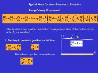
z. x. Typical Mean Dynamic Balances in Estuaries Along-Estuary Component. Steady state, linear motion, no rotation, homogeneous fluid, friction in the vertical only ( A z is a constant). 1. Barotropic pressure gradient vs. friction. The balance can then be rewritten as:. z. x.

E N D
z x Typical Mean Dynamic Balances in Estuaries Along-Estuary Component Steady state, linear motion, no rotation, homogeneous fluid, friction in the vertical only (Az is a constant) 1. Barotropic pressure gradient vs. friction The balance can then be rewritten as:
z x Let’s solve this differential equation; integrating once: Integrating again: This is the solution, but we need two boundary conditions: This makes c1 = 0 Substituting in the solution at z = -H:
General Solution from boundary conditions Particular solution, which can be re-arranged:
expanding the pressure gradient: The momentum balance then becomes: We can write: 2. Pressure gradient vs. vertical mixing O.D.E. with general solution obtained from integrating twice:
General solution: c1and c2 are determined with boundary conditions: This gives the solution: Third degree polynomial proportional to depth and inversely proportional to friction. Requires knowledge of I, G, and wind stress.
We can express I in terms of River Discharge R, G ,and wind stress if we restrict the solution to: Integrating u(z) and making it equal to R, we obtain: Which makes: i.e., the river transport per unit width provides the water added to the system. Note that the effects of G and R are in the same direction, i.e., increase I. The wind stress tends to oppose I.
Substituting into: We get: Density-induced: sensitive to H and Az; third degree polynomial - two inflection points River induced: sensitive to H; parabolic profile Wind-induced: sensitive to H (dubious) and Az; parabolic profile
If we take no bottom stress at z = -H (instead of u(-H) = 0):
Geyer et al (2000) approximations: UTis the tidal current amplitude UE is the magnitude of the estuarine circulation. Also considering that the surface slope scales in proportion to the baroclinic pressure gradient, the momentum eqn becomes where ao is an O (1) constant related to the vertical variability of stress. Momentum balance, steady with friction (tidally averaged)
UE -UE solving for UE where ao0.3 based on Hudson data. (Its value depends on whether the layer average or the maximum is considered).
(2000, JPO, 30, 2035) ao0.3 on Hudson
River z isopycnals Ocean x What drives Gravitational Circulation? Pressure Gradient isobars?
x surface h1 u1 interface U2 = 0 z At interface: At lower layer: 3. Advection vs. Pressure Gradient Take: Upper layer homogeneous and mobile Lower layer immobile Consider inertial effects Ignore friction @ lower layer there is no horizontal pressure gradient The interface slope is of opposite sign to the surface slope
x surface h1 u1 interface But U2 = 0 z The basic balance of forces is Over a volume enclosing the upper layer: Using Leibnitz rule for differentiation under an integral (RHS of last equation; see Officer ((1976), p. 103) we get: This is the momentum balance integrated over the entire upper layer (i.e., energy balance) The quantity inside the brackets (kinetic and potential energy) must remain constant
x Defining transport per unit width: surface h1 u1 interface U2 = 0 Total energy (Kinetic plus Potential energy) remains constant along the system z Differentiating with Respect to ‘q1’ If the density ρ1and the g’ do not change much along the system, we can estimate the changes in h1 as a function of q1 (i.e. how upper layer depth changes with flow)
z z h1 h1 supercritical flow subcritical flow Subcritical flow causes and supercritical flow causes x x This results from a flow slowing down as it moves to deeper regions or accelerating as it moves to shallower waters or through constrictions
Apparent PARADOX!? i.e., u proportional to H 2 This can also be seen from scaling the balance: If we include non-linear terms: Which may be scaled as: i.e., U proportional to H -2 !!! Pressure gradient vs. friction: Ahaa! If L is very large, we go back to u proportional to H 2 Physically, this tells us that when L is small enough the non-linear terms are relevant to the dynamics and the strongest flow will develop over the shallowest areas (fjords). When frictional effects are more important than inertia, then the strongest flow appears over the deepest areas (coastal plain estuaries)!!!
Alternatively: This competition inertia vs. friction to balance the pressure gradient can be explored with a non-dimensional number: When this ratio > 1, inertia dominates When the ratio < 1, friction dominates When H / L > Cb, inertia dominates When H / L < Cb, friction dominates
Similar situation as before (advection vs. presure gradient) but with interfacial friction (fi). Flow in the lower layer but interface remains. There is frictional drag between the two layers. The drag slows down the upper layer and drives a weak flow in the lower layer. x surface h1 u1 interface u2 h2 z In the upper layer, over a volume enclosing the layer: The momentum balance becomes (Officer, 1976; pp. 106-107): 4. Surface Pressure + Advection vs. Interfacial Friction
In the lower layer, the balance is: x The solution has a parabolic shape Boundary conditions: u1 = u2 at the interface u2 =0 at the bottom, z = -H surface h1 u1 interface u2 h2 z u because interface touches the bottom Salt-wedge z
Typical Mean Momentum Balances Barotropic pressure gradient vs. Friction Rivers, Homogeneous Estuaries Total pressure gradient vs. Friction Partially Mixed Estuaries Total pressure gradient vs. Advection Fjords Total pressure gradient vs. Advection + Interfacial Friction Salt Wedge