Download
1 / 68
690 likes | 846 Vues
COSC 3101A - Design and Analysis of Algorithms 3. Recurrences Master’s Method Heapsort and Priority Queue. Many of the slides are taken from Monica Nicolescu’s slides, Univ. Nevada, Reno, monica@cs.unr.edu. Fibonacci numbers. Leonardo Pisano

E N D
COSC 3101A - Design and Analysis of Algorithms3 Recurrences Master’s Method Heapsort and Priority Queue Many of the slides are taken from Monica Nicolescu’s slides, Univ. Nevada, Reno, monica@cs.unr.edu
Fibonacci numbers Leonardo Pisano Born: 1170 in (probably) Pisa (now in Italy)Died: 1250 in (possibly) Pisa (now in Italy) • F(n) = F(n-1) + F(n-2) • F(1) = 0, F(2) = 1 • F(3) = 1, F(4) = 2, F(5) = 3, and so on 1, 1, 2, 3, 5, 8, 13, 21, 34, 55, ... “A certain man put a pair of rabbits in a place surrounded on all sides by a wall. How many pairs of rabbits can be produced from that pair in a year if it is supposed that every month each pair begets a new pair which from the second month on becomes productive? “ COSC3101A
Review: Recursive Algorithms • A recursive algorithm is an algorithm which solves a problem by repeatedly reducing the problem to a smaller version of itself .. until it reaches a form for which a solution exists. • Compared with iterative algorithms: • More memory • More computation • Simpler, natural way of thinking about the problem COSC3101A
Review: Recursive Example (1) N! (N factorial) is defined for positive values as: N! = 0 if N = 0 N! = N * (N-1) * (N-2) * (N-3) * … * 1 if N > 0 For example: 5! = 5*4*3*2*1 = 120 3! = 3*2*1 = 6 The definition of N! can be restated as: N! = N * (N-1)! Where 0! = 1 This is the same N!, but it is defined by reducing the problem to a smaller version of the original (hence, recursively). COSC3101A
Review: Recursive Example (2) int factorial(int num){ if (num == 0) return 1; else return num * factorial(num – 1); } Assume that factorial is called with the argument 4: Call to factorial(4) will return 4 * value returned by factorial(3) Call to factorial(3) will return 3 * value returned by factorial(2) Call to factorial(2) will return 2 * value returned by factorial(1) Call to factorial(1) will return 1 * value returned by factorial(0) Call to factorial(0) returns 1 COSC3101A
Review: Recursive Example (3) The call to factorial(0) has returned, so now factorial(1) can finish: Call to factorial(1) returns 1 * value returned by factorial(0) 1 => 1 The call to factorial(1) has returned, so now factorial(2) can finish: Call to factorial(2) returns 2 * value returned by factorial(1) 1 => 2 The call to factorial(2) has returned, so now factorial(3) can finish: Call to factorial(3) returns 3 * value returned by factorial(2) 2 => 6 The call to factorial(3) has returned, so now factorial(4) can finish: Call to factorial(4) returns 4 * value returned by factorial(3) 6=>24 recursion results in a large number of ‘activation records’ (one per method call) being placed on the system stack COSC3101A
Recurrences Def.: Recurrence = an equation or inequality that describes a function in terms of its value on smaller inputs, and one or more base cases E.g.: Fibonacci numbers: • Recurrence: F(n) = F(n-1) + F(n-2) • Boundary conditions: F(1) = 0, F(2) = 1 • Compute: F(3) = 1, F(4) = 2, F(5) = 3, and so on In many cases, the running time of an algorithm is expressed as a recurrence! COSC3101A
Recurrences and Running Time • Recurrences arise when an algorithm contains recursive calls to itself • What is the actual running time of the algorithm? • Need to solve the recurrence • Find an explicit formula of the expression (the generic term of the sequence) COSC3101A
Typical Recurrences Running Time • T(n) = T(n-1) + n Θ(n2) • Recursive algorithm that loops through the input to eliminate one item • T(n) = T(n/2) + c Θ(lgn) • Recursive algorithm that halves the input in one step • T(n) = T(n/2) + n Θ(n) • Recursive algorithm that halves the input but must examine every item in the input • T(n) = 2T(n/2) + 1 Θ(n) • Recursive algorithm that splits the input into 2 halves and does a constant amount of other work COSC3101A
Recurrences - Intuition • For a recurrence of the type: • It takes f(n) to make the processing for the problem of size n • The algorithm divides the problem into a subproblems, each of size n/b • T(n) = number of subproblems * Running time(n/b) + processing of the problem of size n COSC3101A
Methods for Solving Recurrences • Iteration Method • Substitution Method • Recursion Tree Method • Master Method COSC3101A
Iteration Method • Expand (iterate) the recurrence • Express The function as a summation of terms dependent only on n and the initial condition COSC3101A
Iteration Method – Example(1) T(n) = c + T(n/2) T(n) = c + T(n/2) T(n/2) = c + T(n/4) = c + c + T(n/4) T(n/4) = c + T(n/8) = c + c + c + T(n/8) Assume n = 2k T(n) = c + c + … + c + T(1) = clgn + T(1) = Θ(lgn) k times COSC3101A
Iteration Method – Example(2) T(n) = n + 2T(n/2) T(n) = n + 2T(n/2) T(n/2) = n/2 + 2T(n/4) = n + 2(n/2 + 2T(n/4)) = n + n + 4T(n/4) = n + n + 4(n/4 + 2T(n/8)) = n + n + n + 8T(n/8) … = in + 2iT(n/2i) = kn + 2kT(1) = nlgn + nT(1) = Θ(nlgn) Assume: n = 2k COSC3101A
Substitution method (1) • Guess a solution • Experiences, creativity • iteration method, recursion-tree method • Use induction to prove that the solution works COSC3101A
Substitution method (2) • Guess a solution • T(n) = O(g(n)) • Induction goal: apply the definition of the asymptotic notation • T(n) ≤ c g(n), for some c > 0 and n ≥ n0 • Induction hypothesis: T(k) ≤ c g(k) for all k ≤ n • Prove the induction goal • Use the induction hypothesis to find some values of the constants c and n0 for which the induction goal holds COSC3101A
Substitution Method – Example 1-1 T(n) = T(n-1) + n • Guess: T(n) = O(n2) • Induction goal: T(n) ≤ c n2, for some c and n ≥ n0 • Induction hypothesis: T(k) ≤ ck2 for all k ≤ n • Proof of induction goal: T(n) = T(n-1) + n ≤ c (n-1)2 + n = cn2 – (2cn – c - n) ≤ cn2 if: 2cn – c – n ≥ 0 c ≥ n/(2n-1) c ≥ 1/(2 – 1/n) • For n ≥ 1 2 – 1/n ≥ 1 any c ≥ 1 will work COSC3101A
Substitution Method – Example 1-2 T(n) = T(n-1) + n • Boundary conditions: • Base case: n0 = 1 T(1) = 1 has to verify condition: T(1) ≤ c (1)2 1 ≤ c OK! • We can similarly prove that T(n) = (n2)<your practice> • And therefore: T(n) = (n2) COSC3101A
Substitution Method – Example 2-1 T(n) = 2T(n/2) + n • Guess: T(n) = O(nlgn) • Induction goal: T(n) ≤ cn lgn, for some c and n ≥ n0 • Induction hypothesis: T(n/2) ≤ cn lg(n/2) • Proof of induction goal: T(n) = T(n/2) + n ≤ 2c (n/2)lg(n/2) + n = cn lgn – cn + n ≤ cn lgn if: - cn + n ≤ 0 c ≥ 1 COSC3101A
Substitution Method – Example 2-2 T(n) = 2T(n/2) + n • Boundary conditions: • Base case: n0 = 1 T(1) = 1 has to verify condition: T(1) ≤ cn0lgn0 1 ≤ c * 1 * lg1 = 0 – contradiction • Choose n0 = 2 T(2) = 4 has to verify condition: T(2) ≤ c * 2 * lg2 4 ≤ 2c choose c = 2 • We can similarly prove that T(n) = (nlgn)<your practice> • And therefore: T(n) = (nlgn) COSC3101A
Changing variables T(n) = 2T( ) + lgn • Rename: m = lgn n = 2m T (2m) = 2T(2m/2) + m • Rename: S(m) = T(2m) S(m) = 2S(m/2) + m S(m) = O(mlgm) (demonstrated before) T(n) = T(2m) = S(m) = O(mlgm)=O(lgnlglgn) Idea: transform the recurrence to one that you have seen before COSC3101A
Recursion-tree method Convert the recurrence into a tree: • Each node represents the cost incurred at various levels of recursion • Sum up the costs of all levels Used to “guess” a solution for the recurrence COSC3101A
W(n) = 2W(n/2) + n2 Subproblem size at level i is: n/2i Subproblem size hits 1 when 1 = n/2i i = lgn Cost of the problem at level i = n2/2iNo. of nodes at level i = 2i Total cost: W(n) = O(n2) Recursion-tree Example 1 COSC3101A
Recursion-tree Example 2 E.g.:T(n) = 3T(n/4) + cn2 • Subproblem size at level i is: n/4i • Subproblem size hits 1 when 1 = n/4i i = log4n • Cost of a node at level i = c(n/4i)2 • Number of nodes at level i = 3i last level has 3log4n = nlog43nodes • Total cost: T(n) = O(n2) COSC3101A
regularity condition Master method • “Cookbook” for solving recurrences of the form: where, a ≥ 1, b > 1, and f(n) > 0 Case 1: if f(n) = O(nlogba-) for some > 0, then: T(n) = (nt) Case 2: if f(n) = (nlogba), then: T(n) = (nlogba lgn) Case 3: if f(n) = (nlogba+) for some > 0, and if af(n/b) ≤ cf(n) for some c < 1 and all sufficiently large n, then: T(n) = (f(n)) COSC3101A
Why nlogba? • Case 1: • If f(n) is dominated by nlogba: • T(n) = (nlogbn) • Case 3: • If f(n) dominates nlogba: • T(n) = (f(n)) • Case 2: • If f(n) = (nlogba): • T(n) = (nlogba logn) • Assume n = bk k = logbn • At the end of iteration i = k: COSC3101A
Examples (1) T(n) = 2T(n/2) + n a = 2, b = 2, log22 = 1 Comparenlog22withf(n) = n f(n) = (n) Case 2 T(n) = (nlgn) COSC3101A
Examples (2) T(n) = 2T(n/2) + n2 a = 2, b = 2, log22 = 1 Comparenwithf(n) = n2 f(n) = (n1+) Case 3 verify regularity cond. a f(n/b) ≤ c f(n) 2 n2/4 ≤ c n2 c = ½ is a solution (c<1) T(n) = (n2) COSC3101A
Examples (3) T(n) = 2T(n/2) + a = 2, b = 2, log22 = 1 Comparen withf(n) = n1/2 f(n) = O(n1-) Case 1 T(n) = (n) COSC3101A
Examples (4) T(n) = 3T(n/4) + nlgn a = 3, b = 4, log43 = 0.793 Comparen0.793 withf(n) = nlgn f(n) = (nlog43+)Case 3 Check regularity condition: 3(n/4)lg(n/4) ≤ (3/4)nlgn = c f(n), c=3/4 T(n) = (nlgn) COSC3101A
Examples (5) T(n) = 2T(n/2) + nlgn a = 2, b = 2, log22 = 1 • Compare n with f(n) = nlgn • seems like case 3 should apply • f(n) must be polynomially larger by a factor of n • In this case it is only larger by a factor of lgn COSC3101A
A Job Scheduling Application • Job scheduling • The key is the priority of the jobs in the queue • The job with the highest priority needs to be executed next • Operations • Insert, remove maximum • Data structures • Priority queues • Ordered array/list, unordered array/list COSC3101A
Example COSC3101A
PQ Implementations & Cost Worst-case asymptotic costs for a PQ with N items Insert Remove max ordered array N 1 ordered list N 1 unordered array 1 N unordered list 1 N Can we implement both operations efficiently? COSC3101A
Background on Trees • Def:Binary tree = structure composed of a finite set of nodes that either: • Contains no nodes, or • Is composed of three disjoint sets of nodes: a root node, a left subtree and a right subtree root 4 Right subtree Left subtree 1 3 2 16 9 10 14 8 COSC3101A
4 4 1 3 1 3 2 16 9 10 2 16 9 10 14 8 7 12 Complete binary tree Full binary tree Special Types of Trees • Def:Full binary tree = a binary tree in which each node is either a leaf or has degree exactly 2. • Def:Complete binary tree = a binary tree in which all leaves have the same depth and all internal nodes have degree 2. COSC3101A
The Heap Data Structure • Def:A heap is a nearly complete binary tree with the following two properties: • Structural property: all levels are full, except possibly the last one, which is filled from left to right • Order (heap) property: for any node x Parent(x) ≥ x 8 It doesn’t matter that 4 in level 1 is smaller than 5 in level 2 7 4 5 2 Heap COSC3101A
Definitions • Height of a node = the number of edges on a longest simple path from the node down to a leaf • Depth of a node = the length of a path from the root to the node • Height of tree = height of root node = lgn, for a heap of n elements Height of root = 3 4 1 3 Height of (2)= 1 Depth of (10)= 2 2 16 9 10 14 8 COSC3101A
Array Representation of Heaps • A heap can be stored as an array A. • Root of tree is A[1] • Left child of A[i] = A[2i] • Right child of A[i] = A[2i + 1] • Parent of A[i] = A[ i/2 ] • Heapsize[A] ≤ length[A] • The elements in the subarray A[(n/2+1) .. n] are leaves • The root is the maximum element of the heap A heap is a binary tree that is filled in order COSC3101A
Heap Types • Max-heaps (largest element at root), have the max-heap property: • for all nodes i, excluding the root: A[PARENT(i)] ≥ A[i] • Min-heaps (smallest element at root), have the min-heap property: • for all nodes i, excluding the root: A[PARENT(i)] ≤ A[i] COSC3101A
Operations on Heaps • Maintain the max-heap property • MAX-HEAPIFY • Create a max-heap from an unordered array • BUILD-MAX-HEAP • Sort an array in place • HEAPSORT • Priority queue operations COSC3101A
Operations on Priority Queues • Max-priority queues support the following operations: • INSERT(S, x): inserts element x into set S • EXTRACT-MAX(S): removes and returns element of S with largest key • MAXIMUM(S): returns element of S with largest key • INCREASE-KEY(S, x, k): increases value of element x’s key to k (Assume k ≥ x’s current key value) COSC3101A
Maintaining the Heap Property • Suppose a node is smaller than a child • Left and Right subtrees of i are max-heaps • Invariant: • the heap condition is violated only at that node • To eliminate the violation: • Exchange with larger child • Move down the tree • Continue until node is not smaller than children COSC3101A
Maintaining the Heap Property Alg:MAX-HEAPIFY(A, i, n) • l ← LEFT(i) • r ← RIGHT(i) • ifl ≤ n and A[l] > A[i] • thenlargest ←l • elselargest ←i • ifr ≤ n and A[r] > A[largest] • thenlargest ←r • iflargest i • then exchange A[i] ↔ A[largest] • MAX-HEAPIFY(A, largest, n) • Assumptions: • Left and Right subtrees of i are max-heaps • A[i] may be smaller than its children COSC3101A
A[2] violates the heap property A[4] violates the heap property Heap property restored Example MAX-HEAPIFY(A, 2, 10) A[2] A[4] A[4] A[9] COSC3101A
MAX-HEAPIFY Running Time • Intuitively: • A heap is an almost complete binary tree must process O(lgn) levels, with constant work at each level • Running time of MAX-HEAPIFY is O(lgn) • Can be written in terms of the height of the heap, as being O(h) • Since the height of the heap is lgn COSC3101A
Alg:BUILD-MAX-HEAP(A) n = length[A] fori ← n/2downto1 do MAX-HEAPIFY(A, i, n) Convert an array A[1 … n] into a max-heap (n = length[A]) The elements in the subarray A[(n/2+1) .. n] are leaves Apply MAX-HEAPIFY on elements from 1 to n/2 1 4 2 3 1 3 4 5 6 7 2 16 9 10 8 9 10 14 8 7 Building a Heap A: COSC3101A
1 1 1 1 4 16 4 4 2 2 3 3 2 3 2 3 14 1 10 3 1 3 1 3 4 4 5 5 6 6 7 7 4 5 6 7 4 5 6 7 8 2 16 7 9 9 10 3 2 16 9 10 14 16 9 10 8 8 9 9 10 10 8 9 10 8 9 10 14 2 8 4 1 7 14 8 7 2 8 7 1 1 4 4 2 3 2 3 1 10 16 10 4 5 6 7 4 5 6 7 14 16 9 3 14 7 9 3 8 9 10 8 9 10 2 8 7 2 8 1 Example: A i = 5 i = 4 i = 3 i = 2 i = 1 COSC3101A
1 4 2 3 1 3 4 5 6 7 2 16 9 10 8 9 10 14 8 7 Correctness of BUILD-MAX-HEAP • Loop invariant: • At the start of each iteration of the for loop, each node i + 1, i + 2,…, n is the root of a max-heap • Initialization: • i = n/2: Nodes n/2+1, n/2+2, …, n are leaves they are the root of trivial max-heaps COSC3101A
1 4 2 3 1 3 4 5 6 7 2 16 9 10 8 9 10 14 8 7 Correctness of BUILD-MAX-HEAP • Maintenance: • MAX-HEAPIFY makes node i a max-heap root and preserves the property that nodes i + 1, i + 2, …, n are roots of max-heaps • Decrementing i in the for loop reestablishes the loop invariant • Termination: • i = 0 each node 1, 2, …, n is the root of a max-heap (by the loop invariant) COSC3101A