Download
1 / 33
330 likes | 368 Vues
Learn about the Floyd-Warshall algorithm and efficient solutions for computing shortest paths in networks. Dynamic programming, recursive solutions, matrix multiplication analogy, and improved running times are discussed. Examples and pseudocode provided for better understanding.

E N D
COSC 3101A - Design and Analysis of Algorithms12 All-Pairs Shortest Paths Matrix Multiplication Floyd-Warshall Algorithm
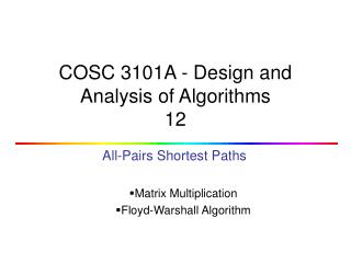
2 4 3 8 1 3 2 1 -4 -5 7 5 4 6 All-Pairs Shortest Paths • Given: • Directed graph G = (V, E) • Weight function w : E → R • Compute: • The shortest paths between all pairs of vertices in a graph • Representation of the result: an n × n matrix of shortest-path distances δ(u, v) COSC3101A
Motivation • Computer network • Aircraft network (e.G. Flying time, fares) • Railroad network • Table of distances between all pairs of cities for a road atlas COSC3101A
All-Pairs Shortest Paths - Solutions • Run BELLMAN-FORD once from each vertex: • O(V2E), which is O(V4) if the graph is dense(E = (V2)) • If no negative-weight edges, could run Dijkstra’s algorithm once from each vertex: • O(VElgV) with binary heap, O(V3lgV) if the graph is dense • We can solve the problem in O(V3) in all cases, with no elaborate data structures COSC3101A
2 4 3 8 1 3 2 1 -4 -5 7 5 4 6 All-Pairs Shortest Paths • Assume the graph (G) is given as adjacency matrix of weights • W = (wij), n x n matrix, |V| = n • Vertices numbered 1 to n if i = j wij = if i j , (i, j) E if i j , (i, j) E • Output the result in an n x n matrix D = (dij), where dij = δ(i, j) • Solve the problem using dynamic programming 0 weight of (i, j) ∞ COSC3101A
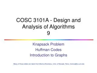
at most m edges 11 j i p’ Optimal Substructure of a Shortest Path • All subpaths of a shortest path are shortest paths • Let p: a shortest path p from vertex i to j that contains at most m edges • If i = j • w(p) = 0 and p has no edges k at most m - 1 edges • If i j:p = i k j • p’ has at most m-1 edges • p’ is a shortest path δ(i, j) = δ(i, k) + wkj COSC3101A
at most m edges 11 j i Recursive Solution • lij(m) = weight of shortest path i j that contains at most m edges • m = 0: lij(0) = if i = j if i j • m 1: lij(m) = • Shortest path from i to j with at most m – 1 edges • Shortest path from i to j containing at most m edges, considering all possible predecessors (k) of j 0 k lij(m-1) min { , } min {lik(m-1) + wkj} 1 k n = min {lik(m-1) + wkj} 1 k n COSC3101A
Computing the Shortest Paths • m = 1: lij(1) = • The path between i and j is restricted to 1 edge • Given W = (wij), compute: L(1), L(2), …, L(n-1), where L(m) = (lij(m)) • L(n-1) contains the actual shortest-path weights Given L(m-1) and W compute L(m) • Extend the shortest paths computed so far by one more edge • If the graph has no negative cycles: all simple shortest paths contain at most n - 1 edges δ(i, j) = lij(n-1) and lij(n), lij(n+1). . . wij L(1) = W = lij(n-1) COSC3101A
j i k k Extending the Shortest Path lij(m)= min {lik(m-1) + wkj} 1 k n j i * = L(m-1) W L(m) n x n Replace: min + + Computing L(m) looks like matrix multiplication COSC3101A
EXTEND(L, W, n) • create L’, an n × n matrix • for i ← 1to n • do for j ← 1to n • do lij’ ←∞ • for k ← 1to n • do lij’ ← min(lij’, lik + wkj) • return L’ Running time: (n3) lij(m)= min {lik(m-1) + wkj} 1 k n COSC3101A
SLOW-ALL-PAIRS-SHORTEST-PATHS(W, n) • L(1) ← W • for m ← 2 to n - 1 • do L(m) ←EXTEND (L(m - 1), W, n) • return L(n - 1) Running time: (n4) COSC3101A
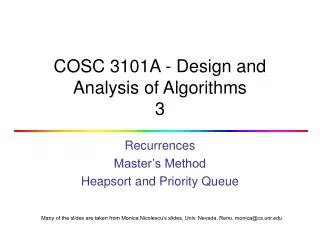
2 4 3 8 1 3 2 1 -4 -5 7 5 4 6 Example W L(m-1) = L(1) 0 3 8 2 -4 3 0 -4 1 7 … and so on until L(4) L(m) = L(2) 4 0 5 11 2 -1 -5 0 -2 8 1 6 0 COSC3101A
Example l14(2) = (0 3 8 -4) 1 0 6 = min (, 4, , , 2) = 2 COSC3101A
Relation to Matrix Multiplication C = a b • cij = Σk=1n aik bkj Compare: D(m) = d(m-1) C dij(m) = min1≤k≤n {dik(m-1) + ckj} COSC3101A
Improving Running Time • No need to compute all L(m) matrices • If no negative-weight cycles exist: L(m) = L(n - 1) for all m n – 1 • We can compute L(n-1) by computing the sequence: L(1) = W L(2) = W2 = W W L(4) = W4 = W2 W2 L(8) = W8 = W4 W4 … COSC3101A
FASTER-APSP(W, n) • L(1) ← W • m ← 1 • while m < n - 1 • do L(2m) ← EXTEND(L(m), L(m), n) • m ← 2m • return L(m) • OK to overshoot: products don’t change after L(n - 1) • Running Time: (n3lg n) COSC3101A
2 4 3 8 1 3 2 1 -4 -5 7 5 4 6 The Floyd-Warshall Algorithm • Given: • Directed, weighted graph G = (V, E) • Negative-weight edges may be present • No negative-weight cycles could be present in the graph • Compute: • The shortest paths between all pairs of vertices in a graph COSC3101A
From A one may reach C faster by traveling from A to B and then from B to C. The Idea COSC3101A
3 6 0.5 1 4 3 2 1 2 5 The Structure of a Shortest Path • Vertices in G are given by V = {1, 2, …, n} • Consider a path p = v1, v2, …, vl • An intermediate vertex of p is any vertex in the set {v2, v3, …, vl-1} • E.g.: p = 1, 2, 4, 5: {2, 4} p = 2, 4, 5: {4} 2 COSC3101A
The Structure of a Shortest Path • For any pair of vertices i, j V, consider all paths from i to j whose intermediate vertices are all drawn from a subset {1, 2, …, k} • Let p be a minimum-weight path from these paths p1 pu j i pt No vertex on these paths has index > k COSC3101A
3 6 0.5 1 2 4 3 2 1 Example dij(k) = the weight of a shortest path from vertex i to vertex j with all intermediary vertices drawn from {1, 2, …, k} • d13(0) = • d13(1) = • d13(2) = • d13(3) = • d13(4) = 6 6 5 5 4.5 COSC3101A
k j i The Structure of a Shortest Path • k is not an intermediate vertex of path p • Shortest path from i to j with intermediate vertices from {1, 2, …, k} is a shortest path from i to j with intermediate vertices from {1, 2, …, k - 1} • k is an intermediate vertex of path p • p1 is a shortest path from i to k • p2 is a shortest path from k to j • k is not intermediary vertex of p1, p2 • p1 and p2 are shortest paths from i to k with vertices from {1, 2, …, k - 1} k j i p1 p2 COSC3101A
A Recursive Solution (cont.) • k = 0 • dij(k) = dij(k) = the weight of a shortest path from vertex i to vertex j with all intermediary vertices drawn from {1, 2, …, k} wij COSC3101A
A Recursive Solution (cont.) dij(k) = the weight of a shortest path from vertex i to vertex j with all intermediary vertices drawn from {1, 2, …, k} • k 1 • Case 1: k is not an intermediate vertex of path p • dij(k) = k j i dij(k-1) COSC3101A
A Recursive Solution (cont.) dij(k) = the weight of a shortest path from vertex i to vertex j with all intermediary vertices drawn from {1, 2, …, k} • k 1 • Case 2: k is an intermediate vertex of path p • dij(k) = k j i dik(k-1) + dkj(k-1) COSC3101A
i j + Computing the Shortest Path Weights • dij(k) = wij if k = 0 min {dij(k-1) , dik(k-1) + dkj(k-1) } if k 1 • The final solution: D(n) = (dij(n)): dij(n) = (i, j) i, j V j (k, j) i (i, k) D(k-1) D(k) COSC3101A
FLOYD-WARSHALL(W) • n ← rows[W] • D(0) ← W • for k ← 1 to n • do for i ← 1 to n • do for j ← 1 to n • do dij(k) ← min (dij(k-1), dik(k-1) + dkj(k-1)) • return D(n) • Running time: (n3) COSC3101A
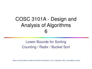
2 0 3 8 -4 4 3 8 0 1 7 1 3 2 4 0 1 -4 -5 7 2 0 5 4 6 6 0 1 2 3 4 5 D(4) D(3) 0 3 8 4 -4 0 3 8 -4 0 3 4 -4 1 0 1 7 0 1 7 0 1 2 4 0 5 11 4 0 4 0 5 3 2 -5 0 -2 2 5 -5 0 -2 2 -1 -5 0 -2 4 6 0 6 0 6 0 5 Example dij(k) = min {dij(k-1) , dik(k-1) + dkj(k-1) } D(1) D(0) = W 1 2 3 4 5 1 2 3 4 5 1 1 2 2 3 3 5 -5 -2 4 4 5 5 D(2) 4 -1 3 -4 -1 5 11 7 3 -1 8 5 1 COSC3101A
D E B C A Transitive Closure • Given a graph G, the transitive closure of G is the G* such that • G* has the same vertices as G • if G has a path from u to v (u v), G* has a edge from u to v D E B G C A The transitive closure provides reachability information about a graph. G* COSC3101A
Transitive Closure of a Directed Graph Def: the transitive closure of G is defined as the graph G*= (V, E*) where E* = {(i,j): there is a path from i to j in G} Given a directed graph G = (V, E) we want to determine if there is a path from i to j for all vertex pairs COSC3101A
Algorithms • The transitive closure can be computed using Floyd-Warshall (i.e. There is a path if ) • There is a more direct approach that can save time in practice and it is very similar to Floyd-Warshall: Let be a boolean value indicting whether there is a path from i to j or not with intermediary vertices in the set { 1,2,…, k}. (I,j) is placed in the set E* iff = 1 ={ 0 if i j and (i, j) E 1 if i = j or (i, j) E COSC3101A
Transitive-Closure Pseudo Code Transitive-Closure(G) (n3) 1 n | V(G)| 2 for i 1 to n 3 do for j 1 to n 4 do if i = j or (i,j) E[G] 5 then tij(0) 1 6 else tij(0) 0 7 for k 1 to n 8 for i 1 to n 9 for j 1 to n 10 11 return T(n) COSC3101A
Readings • Chapter 25 COSC3101A