Download
1 / 13
140 likes | 305 Vues
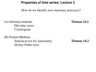
Properties of time series: Lecture 3. How do we identify non-stationary processes? (A) Informal methods Thomas 14.1 Plot time series Correlogram (B) Formal Methods Statistical test for stationarity. Thomas 14.2 Dickey-Fuller tests.

E N D
Properties of time series: Lecture 3 How do we identify non-stationary processes? (A) Informal methods Thomas 14.1 Plot time series Correlogram (B) Formal Methods Statistical test for stationarity. Thomas 14.2 Dickey-Fuller tests.
Informal Procedures to identify non-stationary processes • (1) Eye ball the data (a) Constant mean? • (b) Constant variance?
Informal Procedures to identify non-stationary processes • (2) Diagnostic test - Correlogram • Correlation between 1980 and 1980 + k. • For stationary process correlogram dies out rapidly. • Series has no memory. 1980 is not related to 1985.
Informal Procedures to identify non-stationary processes • (2) Diagnostic test - Correlogram • For a random walk the correlogram does not die out. • High autocorrelation for large values of k
Statistical Tests for stationarity: Simple t-test Set up AR(1) process with drift (α) Xt = α + φXt-1 + ut ut ~ iid(0,σ2) (1) Simple approach is to estimate eqtn (1) using OLS and examine estimated φ {phi} Use a t-test with null Ho: φ = 1 (non-stationary) against alternative Ha: φ < 1 (stationary). Test Statistic: TS = (φ – 1) / (Std. Err.(φ)) reject null hypothesis when test statistic is large negative - 5% critical value is -1.65
Statistical Tests for stationarity: Simple t-test • Simple t-test based on AR(1) process with drift (α) • Xt = α + φXt-1 + ut ut ~ iid(0,σ2) (1) • Problem with simple t-test approach • (1) lagged dependent variables => φ biased downwards in small samples (i.e. dynamic bias) • (2) When φ =1, we have non-stationary process and standard regression analysis is invalid • (i.e. non-standard distribution)
Dickey Fuller (DF) approach to non-stationarity testing • Dickey and Fuller (1979) suggest we subtract Xt-1 from both sides of eqtn. (1) • Xt - Xt-1 = α + φXt-1 - Xt-1 + ut ut ~ iid(0,σ2) • ΔXt = α + φ*Xt-1 + ut φ* = φ –1(2) • Use a t-test with: null Ho: φ* = 0 (non-stationary or Unit Root) • against alternative Ha: φ* < 0 (stationary). • - Large negative test statistics reject non-stationarity • - This is know as unit root test since in eqtn. (1) Ho: φ =1.
Dickey Fuller (DF) tests for unit root • Use t-test with a non-standard distribution because of • (1) dynamic bias in eqtn (1) • (2) non-stationary variables under null • - distribution of Dickey-Fuller test statistics – created by simulation • critical value for τμ-test are larger than normal t-test. τ {tau} • Example • Sample size of n = 25 at 5% level of significance for eqtn. (2) • τμ-critical value = -3.00 t-test critical value = -1.65 • Δpt-1 = -0.007 - 0.190pt-1 • (-1.05) (-1.49) • φ* = -0.190 τμ = -1.49 > -3.00 hence unit root.
Augmented Dickey Fuller (ADF) test for unit root Dickey Fuller tests assume that the residual ut in eqtn. (2) are non-autocorrelated. Solution: incorporate lagged dependent variables. For quarterly data add up to four lags. ΔXt = α + φ*Xt-1 + θ1ΔXt-1 + θ2ΔXt-2 + θ3ΔXt-3 + θ4ΔXt-4 + ut (3) Problem arises of differentiating between models. Use a general to specific approach to eliminate insignificant variables Check final parsimonious model for autocorrelation. Check F-test for significant variables Use Information Criteria. Trade-off parsimony vs residual variance.
Incorporating time trends in ADF test for unit root • From before some time series clearly display an upward trend (non-stationary mean). • Should therefore incorporate trend in ADF test (i.e. equation 3). • ΔXt = α + βtrend + φ*Xt-1 • + θ1ΔXt-1 + θ2ΔXt-2 + θ3ΔXt-3 + θ4ΔXt-4 + ut (4) • It may be the case that Xt will be stationary around a trend. Although if a trend is not included series is non-stationary.
Different DF tests – Summaryt-type test ττΔXt = α + βtrend + φ*Xt-1 + ut (a) Ho:φ*= 0Ha:φ*< 0 τμΔXt = α + φ*Xt-1+ ut (b) Ho: φ* = 0 Ha: φ* < 0 τΔXt = φ*Xt-1 + ut (c)Ho: φ* = 0 Ha: φ* < 0 Critical values from Fuller (1976)
Different DF tests – Summary F-type test Φ3ΔXt = α + βtrend + φ*Xt-1 + ut (a) Ho:φ*= β =0Ha:φ* 0 or β0 Φ1 ΔXt = α + φ*Xt-1+ ut (b) Ho:φ*= α =0Ha:φ* 0 or α0 Critical values from Dickey and Fuller (1981)
Alternative statistical test for stationarity One further approach is the Sargan and Bhargava (1983) test which uses the Durbin-Watson statistic. If Xt is regressed on a constant alone, we then examine the residuals for serial correlation. Serial correlation in the residuals (long memory) will fail the DW test and result in a low value for this test. This test has not proven so popular.