Download
1 / 57
570 likes | 745 Vues
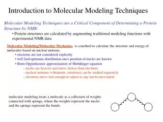
Introduction to Molecular Modeling Techniques. Molecular Modeling Techniques are a Critical Component of Determining a Protein Structure by NMR: Protein structures are calculated by augmenting traditional modeling functions with experimental NMR data.

E N D
Introduction to Molecular Modeling Techniques • Molecular Modeling Techniques are a Critical Component of Determining a Protein Structure by NMR: • Protein structures are calculated by augmenting traditional modeling functions with experimental NMR data • Molecular Modeling/Molecular Mechanicsis a method to calculate the structure and energy of molecules based on nuclear motions. • electrons are not considered explicitly • will find optimum distribution once position of nuclei are known • Born-Oppenheimer approximation of Shrödinger equation • nuclei are heavier and move slower than electrons • nuclear motions (vibrations, rotations) can be studied separately • electrons move fast enough to adjust to any nuclei movement molecular modeling treats a molecule as a collection of weights connected with springs, where the weights represent the nuclei and the springs represent the bonds.
Introduction to Molecular Modeling Techniques • Force Field used to calculate the energy and geometry of a molecule. • Collection of atom types (to define the atoms in a molecule), parameters (for bond lengths, bond angles, etc.) and equations (to calculate the energy of a molecule) • In a force field, a given element may have several atom types. • For example, phenylalanine contains both sp3-hybridized carbons and aromatic carbons. • sp3-Hybridized carbons have a tetrahedral bonding geometry • aromatic carbons have a trigonal bonding geometry. • C-C bond in the ethyl group differs from a C-C bond in the phenyl ring • C-C bond between the phenyl ring and the ethyl group differs from all other C-C bonds in ethylbenzene. The force field contains parameters for these different types of bonds.
Introduction to Molecular Modeling Techniques • Force Field used to calculate the energy and geometry of a molecule. • Total energy of a molecule is divided into several parts called force potentials, or potential • energy equations. • Force potentials are calculated independently, and summed to give the total energy of the • molecule. • Examples of force potentials are the equations for the energies associated with bond stretching, bond bending, torsional strain and van der Waals interactions. • These equations define the potential energy surface of a molecule.
Introduction to Molecular Modeling Techniques • Potential Energy Equation (Bonds Length) • Whenever a bond is compressed or stretched the energy goes up. • The energy potential for bond stretching and compressing is described by an equation • similar to Hooke's law for a spring. • Sum over two atoms • lo – expected/natural bond length • kl – force constant • l – actual/observed bond length Sum over all bonds in the structure From what we know about protein structures what we have been discussing up to this point From the structure Plot of Potential Energy Function for Bond Length
Introduction to Molecular Modeling Techniques • Potential Energy Equation (Angles) • As the bond angle is bent from the norm, the energy goes up. • Sum over three atoms • fo – expected/natural bond angle • kf – force constant • f– actual/observed bond angle Sum over all bond angles in the structure From what we know about protein structures what we have been discussing up to this point From the structure Plot of Potential Energy Function for Bond Angle
Introduction to Molecular Modeling Techniques • Potential Energy Equation (Improper Dihedrals) • As the improper dihedral is bent from the norm, the energy goes up. • Sum over four atoms • wo – expected improper dihedral (usually set to 0o) • kw – force constant • w– actual/observed improper dihedral Sum over all improper dihedrals in the structure Plot of Potential Energy Function for Improper Dihedrals (wo = 0)
Introduction to Molecular Modeling Techniques • Potential Energy Equation (Dihedral Angles) • As the dihedral angle is bent from the norm, the energy goes up. • The torsion potential is a Fourier series that accounts for all 1-4 through-bond • relationships • Sum over four atoms • fo – expected improper dihedral • An – force constant for each Fourier term • – actual/observed improper dihedral n – multiplicity (same parameter seen in the XPLOR constraint file) Sum over all dihedrals in the structure … Fourier Series Plot of Potential Energy Function for Dihedrals Multiple minima
Introduction to Molecular Modeling Techniques • Potential Energy Equation (Dihedral Angles) • Need to include higher terms non-symmetric bonds • Distinguish trans, gauche conformations Different multiplicities identify which torsion angles are energetically equivalent For c1, 60, -60 & 180 are all equivalent and should yield 0 torsion energy
Introduction to Molecular Modeling Techniques • Potential Energy Equation (Nonbonded interactions) • van der waals interaction • Act only at very short distances • Attractive interaction by induced dipoles between uncharged atoms ~r6 • When atoms get too close, valence shell start to overlap and repel ~r12 Van der Waals potential energy function Than becomes repulsive Interaction first attractive
Introduction to Molecular Modeling Techniques • Potential Energy Equation (Nonbonded interactions) • electrostatic interaction • Electrostatic interaction of charged atoms • Long-range forces • Coulomb’s Law Coulomb’s Law Positive interaction that inversely increases distance Negative interaction if of the same charge
Introduction to Molecular Modeling Techniques • Potential Energy Equation (Nonbonded interactions) • electrostatic interaction • Problem defining dielectric constant (e) • dielectric constant differs in solvent and protein interior • eprotein ~ 2-4 • esolvent ~80 • For protein calculations using NMR constraints, typically turn electrostatics off • How to properly define solvent, buffers, salts, etc? • Can explicitly define solvent increases complexity of calculations. • With electrostatics off during the structure calculations, can use the potential energy calculation after the fact to determine the quality of the NMR structure
Introduction to Molecular Modeling Techniques • Potential Energy Equation (Nonbonded interactions) • electrostatic interaction • Problem defining dielectric constant (e) • Don’t use electrostatic potential energy during structure calculation • Use a single dielectric constant • eprotein ~ 2-4; esolvent ~80 • Use explicit solvent in structure calculation • Improved structure quality • Increased computational time • Properly defining solvent • Properly defining force fields behavior in solvent PROTEINS: Structure, Function, and Genetics 50:496–506 (2003)
Introduction to Molecular Modeling Techniques • The Potential Energy Function Not Sufficient to Fold A Protein • it is not even sufficient to keep a folded structure folded. Dynamic simulations, even with the “best” force fields, ALWAYS results in the structure drifting away from the original NMR, X-ray, or homology model GDT-TS – measure of percent similarity to original structure Proteins 2012; 80:2071–2079
Introduction to Molecular Modeling Techniques • Why Is the Potential Energy Function Not Sufficient to Fold A Protein? • It is Not A complete function • primarily short-range geometry with many equal solutions • VDW and electrostatics only contribute over short distances • How do you bring distant regions of the primary chain into contact? • Too many possible conformations • 3N where N is the number of amino acids • Other factors that drive the protein folding process • hydrophobic interactions, hydrogen-bond formation, secondary structure interactions (helix • dipole), effects of solvent, compactness of structure, etc • How do you define a mathematical equation defining these contributions? Improving the Potential Energy Function, improving the parameters and defining alternative ab inito methods of folding a protein are major areas of Molecular Modeling research.
Introduction to Molecular Modeling Techniques • One Way to View an NMR Protein Structure Determination Is as a Hybrid Modeled Structure • NMR structure calculations modify the standard potential energy function to include NMR • experimental constraints • distance constraints (NOEs) • dihedral constraints (NOEs, coupling constants, chemical shifts) • chemical shifts (1H, 13C) • residual dipolar coupling constants (RDCs) • Recently, additional potential functions have been added that are not NMR experimental • constraints but are developed by analyzing databases and structural trends. • Controversial • not true experimental data • but similar to other parameterized geometric functions (bond length, angles etc) • bias structures to structures in PDB • but this is the criteria used to determine the quality of a protein structure ETOTAL = Echem + wexpEexp Eexp = ENOE + Etorsion + EH-bond + Egyr + Erama + ERDC + ECSA + Epara Echem = Ebond + Eangle + Edihedral + Evdw + Eelectr
Introduction to Molecular Modeling Techniques • Ramachandran Database • similar in concept to bond length, bond angle, etc. parameters but directed to f, y, c1 & c2. • based on observed values in the PDB. • Radius of Gyration • based on observed trends in the PDB related to sequence length • tries to improve the compactness of NMR structures • general tendency of a structure in the absence of explicit solvent to move towards an open/expanded chain conformation • Empirical Backbone-Backbone Bonding Potential • based on observed trends in the PDB related to hydrogen bonds in secondary structures and long range isolated H-bonds. • optimizes h-bond distance and angle parameters Convergence of NMR structure
Introduction to Molecular Modeling Techniques • Potential Energy Equation (NMR Constraints) • distance constraint (NOE) • target distance with upper and lower bounds assign ( resid 14 and name HD* ) ( resid 97 and name HD* ) 4.0 2.2 3.0 No contribution to the overall potential energy if the distance between the atoms is between the upper and lower bounds of the NOE constraint
Introduction to Molecular Modeling Techniques . . . noe reset nrestraints = 20000 ceiling 100 class all @noe.tbl averaging all cent potential all square scale all $knoe sqconstant all 1.0 sqexponent all 2 end . . . • Potential Energy Equation (NMR Constraints) • distance constraint (NOE) • Sample XPLOR Script assign ( resid 2 and name HA ) ( resid 2 and name HG2# ) 4.0 2.2 1.6assign ( resid 2 and name HA ) ( resid 3 and name HN ) 2.5 0.7 1.0assign ( resid 2 and name HA ) ( resid 3 and name HD1# ) 4.0 2.2 2.0assign ( resid 2 and name HA ) ( resid 3 and name HD2# ) 4.0 2.2 2.0assign ( resid 2 and name HA ) ( resid 100 and name HB# ) 4.0 2.2 2.0assign ( resid 2 and name HG2# ) ( resid 3 and name HN ) 4.0 2.2 2.0assign ( resid 2 and name HG2# ) ( resid 3 and name HD* ) 4.0 2.2 4.4assign ( resid 2 and name HG2# ) ( resid 100 and name HB# ) 4.0 2.2 3.0assign ( resid 2 and name HG2# ) ( resid 103 and name HN ) 4.0 2.2 2.0 . . . Sets-up the NOE target function and clears any existing constraints Defines the number of constraints and sets the maximal violation energy for a single constraint Assigns a class name to constraints and reads in file containing distance constraints. Can read in multiple files with different class labels. Allows flexibility to treat different classes of NOEs differently. Defines how distances and energies are calculated Which NOE class
Introduction to Molecular Modeling Techniques • Potential Energy Equation (NMR Constraints) • distance constraint (NOE) • Sample XPLOR Script • Averaging – determines how the distance between the selected sets of atoms (pseudoatoms) is calculated. Scaling factor for ambiguous peaks in symmetric multimers R-6 dependence of NOE AVERAGE = R-6 AVERAGE = R-3 AVERAGE = SUM Average of all possible distance combinations Eq. if two distances 3 and 10 Å ((3-6 + 10-6)/2)-1/6 = 3.37 Å Sum of all possible distance combinations Eq. if two distances 3 and 10 Å (3-6 + 10-6)-1/6 = 2.99 Å SUM is preferred over R-6 for ambiguous NOESY crosspeaks AVERAGE = CENTER Difference between geometric centers of atoms (distance constraints have to be corrected for center averaging)
Introduction to Molecular Modeling Techniques • Potential Energy Equation (NMR Constraints) • distance constraint (NOE) • Sample XPLOR Script • Averaging Which is Best (R-6, SUM,CENTER)? Point of Discussion in NMR Community Different upper/lower limits from Val H’s to Hg1 depending on various distance averaging
Introduction to Molecular Modeling Techniques • Potential Energy Equation (NMR Constraints) • distance constraint (NOE) • Sample XPLOR Script • Potential – determines how the energies are calculated for violations of the distance constraints • Square-Well Function is commonly used • scale – determines magnitude of function (force constant) typically 20-50 kcal/mole • ceiling– maximum violation energy per constraint Soft-Square Function Square-Well Function Biharmonic Function Switch point Same flat region around target distance but violation energy for upper violations are reduced at a “switch” point. Energy violation for any distance outside target distance Flat region around target distance where violation energy is zero. Equal energy for upper/lower violations
Introduction to Molecular Modeling Techniques • Potential Energy Equation (NMR Constraints) • distance constraint (NOE) • An even “softer” approach suggests refinement directly against intensities based on a log-normal distribution • IMPORTANT - measurements are not weighted equally but are penalized depending on the degree of disagreement with the structure • No difference for refinements against intensities or distance J. Am. Chem. Soc. (2005) 127, 16026
Introduction to Molecular Modeling Techniques • Potential Energy Equation (NMR Constraints) • Dihedral Angle Restraints • target dihedral angle with upper and lower bounds • similar to NOE square-well function • difference in dihedral angle (f) has to account for circular nature (0-360o) of angles • Force constant (C) – determines the magnitude of the violation energies • Scale (S) – overall weight factor (allows for changes in contribution to overall violation energy during structure calculation • Exponent (ed)– increases violation energies for larger differences in dihedral angles, usually 2 for harmonics. assign (resid 1 and name c ) (resid 2 and name n ) (resid 2 and name ca ) (resid 2 and name c ) 1.0 -93.57 30.0 2
Introduction to Molecular Modeling Techniques . . . restraints dihed reset scale $kcdi nass = 10000 set message off echo off end @dihed.tbl set message on echo on end end . . . • Potential Energy Equation (NMR Constraints) • Dihedral constraints • Sample Xplor script !! g2 assign (resid 1 and name c ) (resid 2 and name n ) (resid 2 and name ca) (resid 2 and name c ) 1.0 70.0 20.0 2 !! k3 assign (resid 2 and name c ) (resid 3 and name n ) (resid 3 and name ca) (resid 3 and name c ) 1.0 60.0 30.0 2 !! f4 assign (resid 3 and name c ) (resid 4 and name n ) (resid 4 and name ca) (resid 4 and name c ) 1.0 -55.0 20.0 2 !! s5 assign (resid 4 and name c ) (resid 5 and name n ) (resid 5 and name ca) (resid 5 and name c ) 1.0 -65.0 30.0 2 !! q6 assign (resid 5 and name c ) (resid 6 and name n ) (resid 6 and name ca) (resid 6 and name c ) 1.0 -70.0 20.0 2 !! t7 assign (resid 6 and name c ) (resid 7 and name n ) (resid 7 and name ca) (resid 7 and name c ) 1.0 -105.0 30.0 2 . . . Sets-up the dihedral target function and clears any existing constraints Defines the number of constraints and sets the maximal violation energy for a single constraint Reads in file containing dihedral constraints. Turns off message so Xplor output file doesn’t contain the reading of all the constraints
Introduction to Molecular Modeling Techniques • Potential Energy Equation (NMR Constraints) • Other NMR empirical constraints follow the same pattern as the NOE and dihedral angles • a difference between the target and observed value determines a violation • a force constant to scale the energy associated with the violation Coupling Constants: Residual Dipolar Coupling Constants: Radius of Gyration:
Introduction to Molecular Modeling Techniques . . . couplings nres 400 potential harmonic class phi degen 1 force 1.0 set echo off message off end coefficients 6.98 -1.38 1.72 -60.0 @coup.tbl class gly !for gly, don't know stereoassignement degen 2 force 1.0 0.2 coefficients 6.98 -1.38 1.72 -60.0 @gly_coup.tbl set echo on message on end end . . . ! T7 assign (resid 6 and name c ) (resid 7 and name n ) (resid 7 and name ca) (resid 7 and name c ) 9.7 0.5 ! C8 assign (resid 7 and name c ) (resid 8 and name n ) (resid 8 and name ca) (resid 8 and name c ) 9.6 0.5 ! Y9 assign (resid 8 and name c ) (resid 9 and name n ) (resid 9 and name ca) (resid 9 and name c ) 8.0 0.5 ! N10 assign (resid 9 and name c ) (resid 10 and name n ) (resid 10 and name ca) (resid 10 and name c ) 7.5 0.5 ! S11 assign (resid 10 and name c ) (resid 11 and name n ) (resid 11 and name ca) (resid 11 and name c ) 5.4 0.5 ! A12 assign (resid 11 and name c ) (resid 12 and name n ) (resid 12 and name ca) (resid 12 and name c ) 8.0 0.5 . . . • Potential Energy Equation (NMR Constraints) • Coupling constant constraints • Sample Xplor script Sets-up the coupling target function defines maximum number of constraints and energy function shape (like NOE) Defines the force constant , degeneracy and coefficients and reads in the experimental constraint files Same for Gly residues, two HA protons, don’t know which is HA1 or HA2. Degeneracy accounts for this
Introduction to Molecular Modeling Techniques . . . collapse assign (resid 1:111) 100.0 12.67 scale 1.0 end . . . • Potential Energy Equation (NMR Constraints) • Radius of Gyration • Sample Xplor script Radius of gyration Force constant ([2.2*(number residues)0.38]-0.5) Turns on the radius of target function Function will be applied to this residue range
Introduction to Molecular Modeling Techniques • Potential Energy Equation (NMR Constraints) • Empirical Backbone-Backbone Hydrogen Bond Constraints • based on an empirical formula derived from high quality X-ray structures in the PDB • violation energy is based on deviations from expected h-bond length (R) and angle (f) Violation occurs if this term is not zero (relationship between R and f)
Introduction to Molecular Modeling Techniques • Potential Energy Equation (NMR Constraints) • Empirical Backbone-Backbone Hydrogen Bond Constraints • based on an empirical formula derived from high quality X-ray structures in the PDB • violation energy is based on deviations from expected h-bond length (R) and angle (f) . !hb database must be read in after psf file hbdb kdir = 0.20 !force constant for directional term klin = 0.08 !force constant for linear term (ca. Nico's hbda) nseg = 1 ! number of segments that hbdb term is active on nmin = 11 !range of residues (number of 1st residue in protein sequence) nmax = 110 !range of residues (number of last residue in protein sequence ) ohcut = 2.60 !cut-off for detection of h-bonds coh1cut = 100.0 !cut-off for c-o-h angle in 3-10 helix coh2cut = 100.0 !cut-off for c-o-h angle for everything else ohncut = 100.0 !cut-off for o-h-n angle updfrq = 10 !update frequency usually 1000 prnfrq = 10 !print frequency usually 1000 freemode = 1 !mode= 1 free search fixedmode = 0 !if you want a fixed list, set fixedmode=1, and freemode=0 mfdir = 0 ! flag that drives HB's to the minimum of the directional potential mflin = 0 ! flag that drives HB's to the minimum of the linearity potential kmfd = 10.0 ! corresp force const kmfl = 10.0 ! corresp force const renf = 2.30 ! forces all found HB's below 2.3 A kenf = 30.0 ! corresponding force const @HBDB:hbdb.inp end . Excerpt of an XPLOR script illustrating how to implement empirical h-bond constraints
Introduction to Molecular Modeling Techniques Expected Cb secondary shifts f-1 f y+1 f+1 y y-1 • Potential Energy Equation (NMR Constraints) • Carbon chemical shift constraint • differences in expected and observed like NOE and dihedral • not a continuous function • “look-up” table with bins (10o) correlating f,y angles with Ca and Cb chemical shifts Bins of expected chemical shift differences (relative to random coil chemical shifts) for Cb chemical shifts plotted as a function of (f,y)
Introduction to Molecular Modeling Techniques . . . carbon phistep=180 psistep=180 nres=300 class all force 0.5 potential harmonic @rcoil.tbl !rcoil shifts @expected_edited.tbl !13C shift database set echo off message off end @carbon.tbl !carbon shifts set echo on message on end end . . . • Potential Energy Equation (NMR Constraints) • Carbon chemical shift constraints • proton chemical shifts setup similarly • Sample Xplor script !! Q6 assign (resid 5 and name c ) (resid 6 and name n ) (resid 6 and name ca) (resid 6 and name c ) (resid 7 and name n ) 57.81 29.28 !! T7 assign (resid 6 and name c ) (resid 7 and name n ) (resid 7 and name ca) (resid 7 and name c ) (resid 8 and name n ) 60.70 69.29 !! C8 assign (resid 7 and name c ) (resid 8 and name n ) (resid 8 and name ca) (resid 8 and name c ) (resid 9 and name n ) 56.57 49.96 !! Y9 assign (resid 8 and name c ) (resid 9 and name n ) (resid 9 and name ca) (resid 9 and name c ) (resid 10 and name n ) 56.53 40.37 !! N10 assign (resid 9 and name c ) (resid 10 and name n ) (resid 10 and name ca) (resid 10 and name c ) (resid 11 and name n ) 53.56 36.29 . . . Sets-up the dihedral target function and number of steps in expectation array Defines the number of constraints, sets the class name (like NOE), the force constant and shape (like NOE) Reads in standard tables for random coil carbon chemical shifts and expected secondary structure chemical shifts Reads in experimental carbon chemical shifts constraint file
Introduction to Molecular Modeling Techniques proton class alpha degeneracy 1 force $kprot error 0.3 @alpha.tbl class gly degeneracy 2 force $kprot $kprotd error 0.3 @alpha_degen.tbl class md degeneracy 2 force $kprot $kprotd error 0.3 @methyl_degen.tbl class ms degeneracy 1 force $kprot error 0.3 @methyl_single.tbl class os degeneracy 1 force $kprot error 0.3 @other_single.tbl class od degeneracy 2 force $kprot $kprotd error 0.3 @other_degen.tbl end • Potential Energy Equation (NMR Constraints) • Proton chemical shift constraints • similar to carbon chemical shifts • Different class (file) for each type of proton • Lists the observed chemical shifts • Degeneracy is dependent on steroassignment • 1 or 2 chemical shifts • Error is conservative uncertainty in chemical shifts • Square-well potential • Sample Xplor script OBSE (resid 10 and (name HA)) 4.414 OBSE (resid 11 and (name HA)) 5.362 OBSE (resid 12 and (name HA)) 4.480 OBSE (resid 13 and (name HA)) 5.022 OBSE (resid 14 and (name HA)) 4.472 OBSE (resid 16 and (name HA)) 4.460 OBSE (resid 17 and (name HA)) 4.480 OBSE (resid 18 and (name HA)) 5.083 OBSE (resid 19 and (name HA)) 5.261 OBSE (resid 20 and (name HA)) 4.320 OBSE (resid 21 and (name HA)) 4.803 . . . Kuszewski et al. (1995) Protein Sci. 107:293
Introduction to Molecular Modeling Techniques • Potential Energy Equation (NMR Constraints) • Ramachandran database constraint • similar to carbon chemical shift constraints • not a continuous function • “look-up” table with bins (8o) correlating f,y, c1 &c2 angles with the probability of occurrence based on PROCHECK analysis of PDB Violation energy is related to the probability of the observed f,y or c1,c2 pair occurring and comparison to neighboring bins. Probability or number of observed occurrences for given pairs of dihedral angles
Introduction to Molecular Modeling Techniques • Potential Energy Equation (NMR Constraints) • Ramachandran database • Sample Xplor script . . . Turns on the Ramachandran database function set message off echo off end rama nres=10000 !intraresidue protein torsion angles @/home/PROGRAMS/xplor-nih-2.9.1/databases/torsions_gaussians/shortrange_gaussians.tbl @/home/PROGRAMS/xplor-nih-2.9.1/databases/torsions_gaussians/new_shortrange_force.tbl !interresidue protein torsion angle correlations i with i+/-1 @/home/PROGRAMS/xplor-nih-2.9.1/databases/torsions_gaussians/longrange_gaussians.tbl @/home/PROGRAMS/xplor-nih-2.9.1/databases/torsions_gaussians/longrange_4D_hstgp_force.tbl end @/home/PROGRAMS/xplor-nih-2.9.1/databases/torsions_gaussians/newshortrange_setup.tbl @/home/PROGRAMS/xplor-nih-2.9.1/databases/torsions_gaussians/setup_4D_hstgp.tbl Automatically sets-up all the expected torsion angles for the protein sequence . . .
Introduction to Molecular Modeling Techniques For a Given Set of Atomic Coordinates, An Energy for the Structure Can Be Calculated Based on the Set of Potential Energy Functions ETOTAL = Echem + wexpEexp Eexp = ENOE + Etorsion + EH-bond + Egyr + Erama + ERDC + ECSA + Epara Echem = Ebond + Eangle + Edihedral + Evdw + Eelectr What Relationship Does This Energy Value Have to Any Experimental Observation? NOTHING! The energy value simply indicates how well the structure conforms to the expected parameters. It does not indicate the relative stability of one protein to another. It does not indicate the stability of the protein (DG). Calculating a DE between the protein with/without a ligand does not indicate the binding affinity of the ligand or the induced stability of the complex Do Not Over Interpret the Meaning of this Energy Function!
Introduction to Molecular Modeling Techniques Consider These Facts About Correctly Folded Proteins: • Typical free energies of protein denaturation (DGd) are ~ 10 kcal/mol • implies the relative stability of the folded protein compared to the denatured (unfolded) protein • In a native structure of a globular protein of 100 amino acids residues there might be: • ~ 100 intramolecular hydrogen bonds • ~ 10 salt links • ~ 10 buried hydrophobic residues • This apparently imparts a stability ca. -1000 kcal/mol to the folded state! • The strength of interactions in the unfolded state must be very similar ( ca. -990 kcal/mol). This suggests that an exceptionally high level of accuracy is needed to correctly analyze energies of different conformers and correctly predict the most stable structure. ETOTAL = Echem + wexpEexp Eexp = ENOE + Etorsion + EH-bond + Egyr + Erama + ERDC + ECSA + Epara Echem = Ebond + Eangle + Edihedral + Evdw + Eelectr We are currently far from this laudable goal.
Introduction to Molecular Modeling Techniques What Relationship Is There Between the Force Constants and Experimental Observations? For geometric parameters (bonds, angles), force constants come from IR, raman spectroscopy and ab inito calculations. For experimental parameters (NOE, dihedral), There is No Relationship! Experimental force constants have been determined by “trial & error” or empirically to obtain a proper balance and weighted contribution of each experimental parameter to the calculated structure.
Introduction to Molecular Modeling Techniques What Do We Mean By a Proper Balance? As example: It is more desirable to have experimental values like NOEs to have more influence on the resulting structure than an empirical function like the Ramachandran database. Thus, the force constant for distance constraints (kNOE) should be higher than the corresponding force constant for the Ramachandran database potential (KDB). . . . evaluate ($knoe = 25.0) ! noes evaluate ($kcdi = 10.0) ! torsion angles evaluate ($kcoup = 1.0) ! coupling constant evaluate ($kcshift = 0.5) ! carbon chemical shifts evaluate ($krgyr = 1.0) ! radius of gyration evaluate ($krama = 1.0) ! intraresidue protein evaluate ($kramalr = 0.15) ! long range protein . . . Typical values of experimental/empirical force constants in XPLOR scripts
Introduction to Molecular Modeling Techniques What Do We Mean By a Proper Balance? These Force Constants Are Not Absolute and Are Routinely Changed During a Structure Calculation . . evaluate ($final_t = 100) { K } evaluate ($tempstep = 50) { K } evaluate ($ncycle = ($init_t-$final_t)/$tempstep) evaluate ($nstep = int($cool_steps*2.5/$ncycle)) evaluate ($bath = $init_t) evaluate ($k_vdw = $ini_con) evaluate ($k_vdwfact = ($fin_con/$ini_con)^(1/$ncycle)) evaluate ($radius= $ini_rad) evaluate ($radfact = ($fin_rad/$ini_rad)^(1/$ncycle)) evaluate ($k_ang = $ini_ang) evaluate ($ang_fac = ($fin_ang/$ini_ang)^(1/$ncycle)) evaluate ($k_imp = $ini_imp) evaluate ($imp_fac = ($fin_imp/$ini_imp)^(1/$ncycle)) evaluate ($noe_fac = ($fin_noe/$ini_noe)^(1/$ncycle)) evaluate ($knoe = $ini_noe) evaluate ($kprot = $ini_prot) evaluate ($prot_fac = ($fin_prot/$ini_prot)^(1/$ncycle)) . . Excerpt of an XPLOR script illustrating how force constants are modified during a structure calculation
Introduction to Molecular Modeling Techniques What Do We Mean By a Proper Balance? Not Only can the Magnitude of the Force Constant be Modified During a Structure Calculation, but Specific Target Functions can be Either Turned Off or On During a Structure Calculation. . . flags exclude * include bonds angles impropers vdw end . . flags exclude * include bond angle dihed impr vdw noe cdih carb rama coup coll end . . Turn off all target function Excerpt of an XPLOR script illustrating how Target Functions are turned off and on. Turn on the selected target function
Introduction to Molecular Modeling Techniques 10 Å H H C C 3 Å H H C C What Do We Mean By a Proper Balance? How can the force constant impact the structure calculation? A Simple Illustration: incorrect distance constraint C-H bond length of 1.1Å with 410 kcal/mol force constant H-H distance constraint of 3.0 Å with 25 kcal/mol force (ceiling of 100 kcal/mol) Distance constraint is violated (properly) with no distortion in bond lengths C-H bond length of 1.1Å with 10 kcal/mol force constant H-H distance constraint of 3.0 Å with 500 kcal/mol force Want to Keep All Known Geometric Values Within Proper Ranges Distance constraint is satisfied (improperly) with large distortion in bond lengths
Introduction to Molecular Modeling Techniques How Do We Use the Energy Function To Calculate a Protein Structure? ETOTAL = Echem + wexpEexp Eexp = ENOE + Etorsion + EH-bond + Egyr + Erama + ERDC + ECSA + Epara Echem = Ebond + Eangle + Edihedral + Evdw + Eelectr Molecular Minimizationstarting from some structure (R), find its potential energy using the potential energy function given above. The coordinate vector R is then varied using an optimization procedure so as to minimize the potential energy ETOTAL(R). Molecular Dynamics the motion of a molecule is simulated as a function of time. Newton's second law of motion is solved to find how the position for each atom of the system varies with time. To find the forces on each atom, the derivative vector (or gradient) of the potential energy function given above is calculated. Factors such as the temperature and pressure of the system can be included in the treatment.
Introduction to Molecular Modeling Techniques Anfinsen's Thermodynamic Hypothesis • The native conformation of a protein is the conformation with the lowest free energy (DG) • global minimum of the free energy surface. • Rather difficult (and expensive) to calculate free energies • by definition these involve averaging over a large number of conformations • Primary sequence determines the protein fold. In 1957, Anfinsen showed that denatured ribonuclease A (124 amino acids, 4 disulphides) produced in 8 M urea and reducing agent (b -mercaptoethanol) could be re-activated by dialysing out the denaturant in oxidizing conditions
Introduction to Molecular Modeling Techniques Levinthal Paradox • If the entire folding process was a random search, it would require too much time • Initial stages of folding must be nearly random. • Conformational changes occur on a time scale of 10-13 seconds. • Proteins are known to fold on a timescale of seconds to minutes. • Consider a 100 residue protein: • if each residue has only 3 possible conformations (far less than reality) 3100 conformation x 10-13 seconds = 1027 years • Even if a significant number of these conformations are sterically disallowed, the folding time would still be astronomical • Energy barriers probably cause the protein to fold along a definite pathway
Introduction to Molecular Modeling Techniques • Molecular Minimization • moves the Cartesian coordinates (X,Y,Z position) for each atom to obtain minimal energy • result is dependent on the starting structure • finds local not global minima • typically, only small movements in atom position are made • starting structure looks similar to ending structure • large changes may occur for significantly distorted structures (stretch bonds) ETOTAL = Echem + wexpEexp Eexp = ENOE + Etorsion + EH-bond + Egyr + Erama + ERDC + ECSA + Epara Echem = Ebond + Eangle + Edihedral + Evdw + Eelectr Large bond change could invert chirality
Introduction to Molecular Modeling Techniques • Molecular Minimization • minimization will fail for severely distorted structures • apoorly docked ligand onto a protein where bonds or atoms are overlapped • In order to properly refine this poor structure, the minimization protocol would need to pull the Cd back through the ring which would require first going to a higher energy structure. • This will not occur since the trend for minimization is to move towards a lower energy. • The “minimized” structure will probably result with a stretched and distorted Cd-Cg bond as it moves the Cd away from the ring from the other direction • the benzene ring and the remainder of the Leu side-chain will also be distorted in an effort to accommodate the overlapped structure Highly unlikely that this structure would minimize since the Cd of the Leu side-chain penetrates the center of the benzene ring
Introduction to Molecular Modeling Techniques Local versus Global Minimum problem Structural landscape is filled with peaks and valleys. Minimization protocol always moves “down hill”. No means to “see” the overall structural landscape No means to pass through higher intermediate structures to get to a lower minima. The initial structure determines the results of the minimization!
Introduction to Molecular Modeling Techniques Local versus Global Minimum problem Another perspective of the Structural Landscape is a 3D funnel view that leads to the global minimum at the base of the funnel.
Introduction to Molecular Modeling Techniques • Molecular Minimization • Process Overview The molecular potential U depends on two types of variables: Potential energy gradient g(Q), a vector with 3N components: The necessary condition for a minimum is that the function gradient is zero: Where xi denote atomic Cartesian coordinates and N is the number of atoms or The sufficient condition for a minimum is that the second derivative matrix is positive definite, i.e. for any 3N-dimensional vector u: A simpler operational definition of this property is that all eigenvalues of F are positive at a minimum. The second derivative matrix is denoted by F in molecular mechanics and H in mathematics, and is defined as: One measure of the distance from a stationary point is the rms gradient:
Introduction to Molecular Modeling Techniques • Molecular Minimization • Process Overview • minima occurs when the first derivative is zero and when the second derivative is positive. • U(Q) is a complicated function varying quickly with atomic coordinates Q • molecular energy minimization is often performed in a series of steps • the coordinates at step n+1 are determined from coordinates at previous step n where dn is called a step. • the initial step is a guess • a systematic or random search is not practical (Levinthal Paradox) • Steepest Descent Method • search step (dn) is performed in the direction of fastest decrease of U, opposite of the gradient g where a is a factor determining the length of the step. • not efficient, but good for initial distorted structures • may be very slow near a solution Always makes right angle


![Data Modeling [Comparison of data modeling techniques ]](https://cdn0.slideserve.com/205866/data-modeling-comparison-of-data-modeling-techniques-dt.jpg)