Advanced Methods in Conduction Modeling and eQUEST Software Overview
This lecture focuses on advanced methods for solving conduction equations with an emphasis on alternative techniques using response function methods. Students will explore the commercial software eQUEST for energy simulation and the basic modeling steps involved. The lecture also covers the latest updates on Homework 3, designed to enhance understanding of unsteady conduction in realistic scenarios. The session includes practical examples and lays the groundwork for future analysis of moisture transport and temperature distribution within wall elements.

Advanced Methods in Conduction Modeling and eQUEST Software Overview
E N D
Presentation Transcript
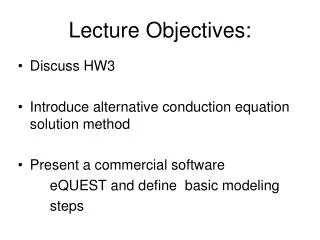
Lecture Objectives: • Discuss HW3 • Introduce alternative conduction equation solution method • Present a commercial software eQUEST and define basic modeling steps
Top view Homework 3 (Similar to HW2, but unsteady, and more realistic) Glass Tnorth_oi Tnorth_i Tinter_surf ≠ Tair 2.5 m Surface radiation Tair_in 10 m IDIR 10 m Teast_i Idif East North Insulation Teast_o Tair_out Concrete Surface radiation Idif IDIR
Alternative: Response function methods for conduction calculation NOTATION: θ(x,t)=T(x,)
Laplace transformation Laplace transform is given by Where p is a complex number whose real part is positive and large enough to cause the integral to converge.
Principles of Response function methods The basic strategy is to predetermine the response of a system to some unit excitation relating to the boundary conditions anticipated in reality. Reference: JA Clarke http://www.esru.strath.ac.uk/Courseware/Class-16458/ or http://www.hvac.okstate.edu/research/documents/iu_fisher_04.pdf
Response functions • Computationally inexpensive • Accuracy ? • Flexibility ???? What if we want to calculate the moisture transport and we need to know temperature distribution in the wall elements?
Modeling 1) External wall (north) node Qsolar+C1·A(Tsky4 - Tnorth_o4)+ C2·A(Tground4 - Tnorth_o4)+hextA(Tair_out-Tnorth_o)=Ak/(Tnorth_o-Tnorth_in) A- wall area [m2] • - wall thickness [m] k – conductivity [W/mK] - emissivity [0-1] • - absorbance [0-1] • = - for radiative-gray surface, esky=1, eground=0.95 Fij –view (shape) factor [0-1] h – external convection [W/m2K] s – Stefan-Boltzmann constant [5.67 10-8 W/m2K4] Qsolar=asolar·(Idif+IDIR)A C1=esky·esurface_long_wave·s·Fsurf_sky C2=eground·esurface_long_wave·s·Fsurf_ground 2) Internal wall (north) node C3A(Tnorth_in4- Tinternal_surf4)+C4A(Tnorth_in4- Twest_in4)+hintA(Tnorth_in-Tair_in)= =kA(Tnorth_out--Tnorth_in)+Qsolar_to_int_ considered _surf Qsolar_to int surf =portion of transmitted solar radiation that is absorbed by internal surface C3=eniort_in·s·ynorth_in_to_ internal surface for homeworkassume yij = Fijei
Modeling b1T1 + +c1T2+=f(Tair,T1,T2) a2T1+b2T2 + +c2T3+=f(T1 ,T2, T3) a3T2+b3T3+ +c3T4+=f(T2 ,T3 , T4) ……………………………….. a6T5+b6T6+ =f(T5 ,T6 , Tair) Matrix equation M × t = f for each time step M × t = f
Modeling steps • Define the domain • Analyze the most important phenomena and define the most important elements • Discretize the elements and define the connection • Write the energy and mass balance equations • Solve the equations (use numeric methods or solver) • Present the result
eQUEST • Energy simulation software • Free: http://doe2.com/equest/ • Graphical user interface (GUI) that uses DOE2 • Easy to use it • Example of your HW1a • ….