Lecture Objectives:
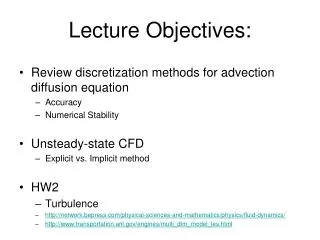
Lecture Objectives:. Review discretization methods for advection diffusion equation Accuracy Numerical Stability Unsteady-state CFD Explicit vs. Implicit method HW2 Turbulence http://network.bepress.com/physical-sciences-and-mathematics/physics/fluid-dynamics/

Lecture Objectives:
E N D
Presentation Transcript
Lecture Objectives: • Review discretization methods for advection diffusion equation • Accuracy • Numerical Stability • Unsteady-state CFD • Explicit vs. Implicit method • HW2 • Turbulence • http://network.bepress.com/physical-sciences-and-mathematics/physics/fluid-dynamics/ • http://www.transportation.anl.gov/engines/multi_dim_model_les.html
Steady–state 1D example I) X direction • If Vx > 0, • If Vx < 0, Convection term - Upwind-scheme: P E W dxe dxw and a) and Dx e w Diffusion term: b) When mesh is uniform: DX = dxe = dxw Assumption: Source is constant over the control volume Source term: c)
Advection diffusion equation 1-D, steady-state Dx Dx N N+1 N-1 Different notation: Dx General equation
1D example multiple (N) volumes N unknowns i N 1 2 N-1 3 Equation for volume 1 N equations Equation for volume 2 …………………………… Equation matrix: For 1D problem 3-diagonal matrix
3D problem Equation in the general format: H N W E P S L Wright this equation for each discretization volume of your discretization domain A F 60,000 elements 60,000 cells (nodes) N=60,000 = x 60,000 elements 7-diagonal matrix This is the system for only one variable ( ) When we need to solve p, u, v, w, T, k, e, C system of equation is very larger
Boundary conditionsfor CFD application - indoor airflow Real geometry Model geometry Where are the boundary Conditions?
CFD ACCURACY Depends on airflow in the vicinity of Boundary conditions 1) At air supply device 2) In the vicinity of occupant 3) At room surfaces • Detailed modeling • limited by • computer power
Surface boundaries thickness 0.01-20 mm for forced convection Wall surface W use wall functions to model the flow in the vicinity of surface Using relatively large mesh (cell) size.
momentum sources Airflow at air supply devices Complex geometry - Δ~10-4m We can spend all our computing power for one small detail
Diffuser jet properties High Aspiration diffuser D D L L How small cells do you need? We need simplified models for diffusers
Simulation of airflow in In the vicinity of occupants How detailed should we make the geometry?
General Transport EquationUnsteady-state H N Equation in the algebraic format: W E P S L We have to solve the system matrix for each time step ! Transient term: Are these values for step or + ? If: - - explicit method - + - implicit method Unsteady-state 1-D
General Transport Equationunsteady-state 1-D Fully explicit method: Implicit method: Value form previous time step (known value) • Make the difference between • - Calculation for different time step • - Calculation in iteration step