Numerical Weather Prediction and Data Assimilation
480 likes | 1.21k Vues
Numerical Weather Prediction and Data Assimilation. David Schultz, Mohan Ramamurthy, Erik Gregow, John Horel. What is a model?. Resource: Kalnay, E., 2003: Atmospheric Modeling, Data Assimilation and Predictability

Numerical Weather Prediction and Data Assimilation
E N D
Presentation Transcript
Numerical Weather Prediction and Data Assimilation David Schultz, Mohan Ramamurthy, Erik Gregow, John Horel
What is a model? • Resource: Kalnay, E., 2003: Atmospheric Modeling, Data Assimilation and Predictability • model: tool for simulating or predicting the behavior of a dynamical system such as the atmosphere • Types of models include: • heuristic: rule of thumb based on experience or common sense • empirical: prediction based on past behavior • conceptual: framework for understanding physical processes based on physical reasoning • analytic: exact solution to “simplified” equations that describe the dynamical system • numerical: integration of governing equations by numerical methods subject to specified initial and boundary conditions
What is Numerical Weather Prediction? • The technique used to obtain an objective forecast of the future weather (up to possibly two weeks) by solving a set of governing equations that describe the evolution of variables that define the present state of the atmosphere. • Feasible only using computers
A Brief History • Recognition by V. Bjerknes in 1904 that forecasting is fundamentally an initial-value problem and basic system of equations already known • L. F. Richardson’s (1922) attempt at practical NWP • Radiosonde invention in 1930s made upper-air data available • Late 1940s: First successful dynamical-numerical forecast made by Charney, Fjortoft, and von Neumann • 1960s: Edward Lorenz shows the atmosphere is chaotic and its predictibility limit is about two weeks
NWP System • NWP entails not just the design and development of atmospheric models, but includes all the different components of an NWP system • It is an integrated, end-to-end forecast process system
Components of an NWP model • 1. Governing equations • F=ma, conservation of mass, moisture, and thermodynamic eqn., gas law • 2. Numerical procedures: • approximations used to estimate each term (especially important for advection terms) • approximations used to integrate model forward in time • boundary conditions • 3. Approximations of physical processes (parameterizations) • 4. Initial conditions: • Observing systems, objective analysis, initialization, and data assimilation
Model Physics • Grid-scale precip. (large scale condensation) • Deep and shallow convection • Microphysics (increasingly becoming important) • Evaporation • PBL processes, including turbulence • Radiation • Cloud-radiation interaction • Diffusion • Gravity wave drag • Chemistry (e.g., ozone, aerosols)
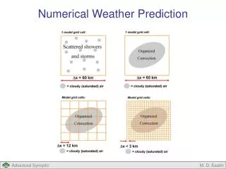
Grid spacing (resolution) defines the scale of the features you can simulate with the model.
Good Numerical Forecasts Require… • Initial conditions that adequately represent the state of the atmosphere (three-dimensional wind, temperature, pressure, moisture and cloud parameters) • Numerical weather prediction model that adequately represents the physical laws of the atmosphere over the whole globe
Sources of error in NWP • Errors in the initial conditions • Errors in the model • Intrinsic predictability limitations • Errors can be random and/or systematic errors
Initial Condition Errors Observational Data Coverage Spatial Density Temporal Frequency Errors in the Data Instrument Errors Representativeness Errors Errors in Quality Control Errors in Objective Analysis Errors in Data Assimilation Missing Variables Model Errors Equations of Motion Incomplete Errors in Numerical Approximations Horizontal Resolution Vertical Resolution Time Integration Procedure Boundary Conditions Horizontal Vertical Terrain Physical Processes Sources of Errors - continued Source: Fred Carr
Given all these assumptions and limitations, we have no right to do as well in forecasting the weather as we do! Dave sez: • What other disciplines forecast the future with as much success as meteorology?
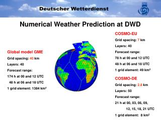
NWP in Finland • Currently, NWP models are run by FMI (limited domain over Europe) and by the European Centre for Medium-Range Weather Forecasts (global) • Currently the FMI model is run at about 9 & 22 km and the ECMWF model is run at 25 km grid spacing, meaning that these models can resolve features about 6 times those grid spacings. • The new AROME experimental model is running at 2.5 km grid spacing.
22 km HIRLAM 9 km HIRLAM 2.5 km AROME
9 km HIRLAM 2.5 km AROME observed radar reflectivity
9 km HIRLAM 2.5 km AROME
The Hopes of the Testbed • Higher-resolution observations will provide higher-resolution initial conditions, which could be put into a higher-resolution NWP model, producing higher-resolution forecasts. • The hope is that precise forecasts of convection, the sea breeze, rain/snow forecasting, and winds could be made up to a few hours in advance. • BUT…
Difficulties Lie Ahead… • The reality is often that you end up with a higher-resolution, less-accurate forecast. • Results from forecasting/research experiments at the NOAA/Storm Prediction Center show value can be added sometimes with high-resolution forecasts. • When that value can be added is a very important forecasting/research question!!!
Difficulties Lie Ahead… • Producing the initial conditions from sparse resolution (in space and time) and incomplete observations is not easy. • Creating a gridded 3-D/4-D dataset suitable for initializing a NWP model is called data assimilation. • How it is proposed to be done in the Helsinki Testbed is described next…
Numerical weather prediction model that adequately represents the physical laws of the atmosphere over the whole globe • Initial conditions that adequately represent the state of the atmosphere (three-dimensional wind, temperature, pressure, moisture and cloud parameters)
Good Numerical Forecasts Require… • Numerical weather prediction model that adequately represents the physical laws of the atmosphere over the whole globe • Initial conditions that adequately represent the state of the atmosphere (three-dimensional wind, temperature, pressure, moisture and cloud parameters)
Monitoring Current Conditions September 6 20GMT A D A S
Potential Discussion Points • Why are analyses needed? • Application driven: data assimilation for NWP (forecasting) vs. objective analysis (specifying the present, or past) • What are the goals of the analysis? • Define microclimates? • Requires attention to details of geospatial information (e.g., limit terrain smoothing) • Resolve mesoscale/synoptic-scale weather features? • Requires good prediction from previous analysis • What’s the current state-of-the-art and what’s likely to be available in the future? • Deterministic analyses relative to ensembles of analyses (“ensemble synoptic analysis”–Greg Hakim) • How is analysis quality determined? What is truth? • Why not rely on observations alone to verify model guidance?
Observations vs. Truth • “Truth? You can’t handle the truth!” • Truth is unknown and depends on application: “expected value for 5 x 5 km2 area” • Assumption: average of many unbiased observations should be same as expected value of truth • However, accurate observations may be biased or unrepresentative due to siting or other factors
x What’s an appropriate analysis given the inequitable distribution of observations? Case 3 Case 2 Case 1 ? ? x ? x x = grid cell = observation
What’s an appropriate analysis given the variety of weather phenomena? Elevated Valley Inversions Front ? O ? O ? O O O O z T
Analyses vs. Truth Analysis value = Background value + observation Correction • An analysis is more than spatial interpolation • A good analysis requires: • a good background field supplied by a model forecast • observations with sufficient density to resolve critical weather and climate features • information on the error characteristics of the observations and background field • good techniques (forward observation operators) to transform the background gridded values into pseudo observations • Analysis error relative to unknown truth should be smaller than errors of observations and background field • Ensemble average of analyses should be closer to truth than single deterministic approach IF the analyses are unbiased
Truth Truth = H(Truth) Truth: Continuum vs. Discrete Truth is unknown Truth depends on application Temperature Truth West East
Truth Analysis Error Analysis Discrete Analysis ErrorGoal of objective analysis: minimize error relative to Truth not Truth! Temperature Truth West East
ADAS • Near-real time surface • analysis of T, RH, V • (Lazarus et al. 2002 WAF; • Myrick et al. 2005 WAF; • Myrick & Horel2006 WAF) • Analyses on NWS GFE • grid at 5 km spacing • Background field: RUC • Horizontal, vertical & anisotropic weighting
Description: In the following slides, temperature results from LAPS/MM5 analysis are shown. The objective is to compare a normal MM5 analysis with LAPS/MM5 analysis, also verify against some observations that are not included into the LAPS analysis Input to LAPS analysis is here: - MM5 9-km resolution (input to MM5 is ECMWF 0.35 deg) - 52 surface observations from HTB area
MM5 analysis: Temperature at 9 m height, with 1 km resolution The analysis is based on 0.35 degree boundary fields from ECMWF operational analysis. 09 Aug 2005,15 UTC
* * 23.7 23.4 23.6 * 22.1 * 23.0 24.3 * * 26.0 * 25.4 * 25.4 23.5 * * 20.5 * 20.4 20.2 * 22.0 * 20.9 * * 20.7 * MM5 analysis: Temperature at 9 m height, with 1 km resolution Verification: The figures, within the plot, are measurements from certain stations not included in the LAPS analysis 09 Aug 2005,15 UTC
* * 23.7 23.4 23.6 * 22.1 * 23.0 24.3 * * 26.0 * 25.4 * 25.4 23.5 * * 20.5 * 20.4 20.2 * 22.0 * 20.9 * * 20.7 * LAPS/MM5 analysis: Temperature at 9 m height, with 3 km resolution Verification: The figures, within the plot, are measurements from certain stations not included in the LAPS analysis 09 Aug 2005,15 UTC
* * 23.7 23.4 23.6 * 22.1 * 23.0 24.3 * * 26.0 * 25.4 * 25.4 23.5 * * 20.5 * 20.4 20.2 * 22.0 * 20.9 * * 20.7 * LAPS/MM5 analysis: Temperature at 9 m height, with 1 km resolution Verification: The figures, within the plot, are measurements from certain stations not included in the LAPS analysis 09 Aug 2005,15 UTC
* * 23.7 23.4 23.6 * 22.1 * 23.0 24.3 * * 26.0 * 25.4 WHAT IS TRUTH? * 25.4 23.5 * * 20.5 * 20.4 20.2 * 22.0 * 20.9 * * 20.7 * LAPS/MM5 analysis: Temperature at 9 m height, with 1 km resolution Verification: The figures, within the plot, are measurements from certain stations which are not included in the LAPS analysis 09 Aug 2005,15 UTC
Data Assimilation Surprises • Torn and Hakim (unpublished) have applied an ensemble Kalman filter for several hurricanes to determine the most sensitive regions for forecasts in the western Pacific Ocean. The largest sensitivities are associated with upper-level troughs upstream of the tropical cyclone. Observation impact calculations indicate that assimilating ~40 key observations can have nearly the same impact on the forecast as assimilating all 12,000 available observations. • Sensitivity of the 48 hour forecast of tropical cyclone minimum central pressure to the analysis of 500 hPa geopotential height (colors) for the forecast initialized 12 UTC 19 October 2004. Regions of warm (cold) colors indicate that increasing the analysis of 500 hPa height at that point will increase (decrease) the 48 hour forecast of minimum central pressure. The contours are the ensemble mean analysis of 500 hPa height.
More Data Assimilation Woes • Adaptive observations: collecting data where the forecast is most sensitive • Sometimes assimilating more data produces a worse forecast (Morss and Emanuel) • Heretical thought: What if none of the hundreds of observations from the Helsinki Testbed made any difference to the forecast?
Challenges Ahead for Testbed/LAPS • The Testbed only samples the lower troposphere at best, not the mid and upper troposphere. • Weather phenomena, even adequately sampled by the Testbed data, will move out of the Testbed domain within an hour or two. • Weather phenomena inadequately sampled by the Testbed data will move into the domain and screw up your forecast. • Predictability of mesoscale weather features is unknown. • All of this assumes a perfect model.
Challenges Ahead for Forecasters • Determinism is dead—long live probabilistic forecasting! • High-resolution model output cannot be interpreted the same way as a coarser-resolution model output. • Forecasters need to be retrained. • Communication of high-resolution forecasts to end users is not simple (i.e., you cannot just send raw model output to users and expect them to use it). • This ensures jobs for good forecasters in the future.