Numerical Weather Prediction: An Overview
Numerical Weather Prediction: An Overview. Mohan Ramamurthy Department of Atmospheric Sciences University of Illinois at Urbana-Champaign E-mail: mohan@uiuc.edu COMET Faculty Course on NWP June 7, 1999. What is Numerical Weather Prediction?.

Numerical Weather Prediction: An Overview
E N D
Presentation Transcript
Numerical Weather Prediction:An Overview Mohan Ramamurthy Department of Atmospheric Sciences University of Illinois at Urbana-Champaign E-mail: mohan@uiuc.edu COMET Faculty Course on NWP June 7, 1999
What is Numerical Weather Prediction? • The technique used to obtain an objective forecast of the future weather (up to possibly two weeks) by solving a set of governing equations that describe the evolution of variables that define the present state of the atmosphere. • Feasible only using computers
A Brief History • Recognition by V. Bjerknes in 1904 that forecasting is fundamentally an initial-value problem and basic system of equations already known • L. F. Richardson’s first attempt at practical NWP • Radiosonde invention in 1930s made upper-air data available • Late 1940s: First successful dynamical-numerical forecast made by Charney, Fjortoft, and von Neumann
NWP System • NWP entails not just the design and development of atmospheric models, but includes all the different components of an NWP system • It is an integrated, end-to-end forecast process system • USWRP focus: “best practicable mix” of observations, data assimilation schemes, and forecast models.
Components of an NWP model • 1. Governing equations • 2. Physical Processes - RHS of equations (e.g., PGF, friction, adiabatic warming, and parameterizations) • 3. Numerical Procedures: • approximations used to estimate each term (especially important for advection terms) • approximations used to integrate model forward in time • boundary conditions • 4. Initial Conditions: • Observing systems, objective analysis, initialization, and data assimilation
Notable Trends • Use of filtered models in early days of NWP • Objective analysis methods • Terrain-following coordinate system • Improved finite-difference methods • Availability of asynoptic data: OSSE and data assimilation issues • Global spectral modeling • Normal mode initialization • Economic integration schemes (e.g., semi-implicit)
Trends - continued • Parameterization of model physics • Model output statistics • Diabatic initialization • Four-dimensional data assimilation • Regional spectral modeling • Introduction of adjoint approach • Ensemble forecasting • Targeted (or adaptive) observations
Computing trends • NWP has evolved as computers have evolved • The big irons: early 1950- late 1970 • Vector supercomputers: Late 1970s • Multi-processors: 1980s • Massively parallel supercomputers • High-performance workstations • Personal computers as workstations
Hierarchy of models • Euler equations • Primitive equation • Hydrostatic vs. Non-hydrostatic • Filtered equations: • Filter out sound and gravity waves • Permits larger time-step for integration • Filtering sound waves: • Incompressible • Anelastic • Boussinesq • Filtering gravity waves: • Quasi-geostrophic • Semi-geostrophic • Equivalent barotropic
Governing Equations • It was recognized early in the history of NWP that primitive equations were best suited for NWP • Governing equations can be derived from the conservation principles and approximations. • It is important for students to understand the resulting wave solutions and their relationship to the chosen approximations. • e. g., shallow-water models: one Rossby mode and two gravity modes
Key Conservation Principles • conservation of motion (momentum) • conservation of mass • conservation of heat (thermodynamic energy) • conservation of water (mixing ratio/specific humidity) in different forms (e.g., Qv, Qr, Qs, Qi, Qg), and • conservation of other gaseous and aerosol materials
Prognostic variables • Horizontal and vertical wind components • Potential temperature • Surface pressure • Specific humidity/mixing ratio • Mixing ratios of cloud water, cloud ice, rain, snow, graupel • PBL depth or TKE • Mixing ratio of chemical species
Vertical Representation • Sigma (terrain following): e.g., NGM, MM5 • Eta (step mountain): Eta model • Theta (isentropic) • Hybrid (sigma-theta): RUC • Hybrid (sigma-z): GEM (Canadian model) • Pressure (no longer popular in NWP) • Height (mostly used in cloud models)
Map projections: Why? • Equations are often cast on projections • Output always displayed on a projection • Data often available on native grids • Projections used in NWP: • Lambert-conformal • Polar stereographic • Mercator • Spherical or Gaussian grid
Numerical Methods • Finite difference (e.g., Eta, RUC-II, and MM5) • Galerkin • Spectral (e.g., MRF, ECMWF, RSM, and all Japanese operational models) • Finite elements (Canadian operational models) • Adaptive grids (COMMAS cloud model)
Time-integration schemes • Two-level (e.g., Forward or backward) • Three-level (e.g., Leapfrog) • Multistage (e.g., Forward-backward) • Higher-order schemes (e.g., Runge-Kutta) • Time splitting (split explicit) • Semi-implicit • Semi-Lagrangian
Numerics: Important considerations • Accuracy and consistency • Stability and convergence • Efficiency • Monotonicity and conservation (e.g., positive definite advection) • Aliasing and Nonlinear instability • Controlling computational mode (e.g., Asselin filter) • Other forms of smoothing (e.g., diffusion)
Eulerian or Semi-Lagrangian? • Efficiency depends on applications • Semi-Lagrangian methods require more calculations per time step • S-L approach advantageous for tracer transport calculations (conservative quantities) • S-L method is superior in models w/ spherical geometry • Problems in which frequency of the forcing is similar in both Lagrangian and Eulerian reference
Eulerian vs. S-L methods - contd • When the frequency of the forcing is similar in both Lagrangian and Eulerian reference frames, S-L approach loses its advantage • S-L can be coupled with Semi-implicit schemes to gain significant computational advantage. • ECMWF model S-L/SI example: • Eulerian approach: 3-min time step • S-L/SI approach: 20-min time step • S-L 400% more efficient including overhead
Staggered Meshes • Spatial staggering (velocity and pressure) • Arakawa grid staggering (horizontal) • Lorenz staggering (vertical) • Wave motions and dispersion properties better represented with certain staggered meshes • e.g., important in geostrophic adjustment • Temporal staggering
Boundary Conditions • Lateral B. C. essential for limited-area models • Top and lower B. C. needed for all models • Some Examples: • Relaxation (Davis, 1976) • Blending (Perkey-Kreitzberg, 1976) • Periodic • Radiation (Orlanski, 1975) • Fixed, symmetric
Model Physics • Grid-scale precip. (large scale condensation) • Deep and shallow convection • Microphysics (increasingly becoming important) • Evaporation • PBL processes, including turbulence • Radiation • Cloud-radiation interaction • Diffusion • Gravity wave drag • Chemistry (e.g., ozone, aeorosols)
Model Performance • Validation • Verification • Skill score, RMS error, AC, ETS, biases, etc. • Verification of probabilistic forecasts • Mesoscale verification problem • QPF verification • Verification over complex terrain
Sources of error in NWP • Errors in the initial conditions • Errors in the model • Intrinsic predictability limitations • Errors can be random and/or systematic errors
Initial Condition Errors Observational Data Coverage Spatial Density Temporal Frequency Errors in the Data Instrument Errors Representativeness Errors Errors in Quality Control Errors in Objective Analysis Errors in Data Assimilation Missing Variables Model Errors Equations of Motion Incomplete Errors in Numerical Approximations Horizontal Resolution Vertical Resolution Time Integration Procedure Boundary Conditions Horizontal Vertical Terrain Physical Processes Sources of Errors - continued Source: Fred Carr
Forecast Error Growth and Predictability Source: Fred Carr
Galerkin Method - Series Expansion Method • The dependent variables are represented by a finite sum of linearly independent basis functions. • Includes: • the spectral method • the pseudospectral method, and • the finite element method • Less widely used in meteorology (ex. Canadian models) • Basis functions are local • Can provide non-uniform grid (resolution)
Spectral Methods • The basis functions are orthogonal • The choice of basis function dictated by the geometry of the problem and boundary conditions. • Introduced in 1954 to meteorology, but it did not become popular until the mid 70s. • Principal advantage: The spectral representation does not introduce phase speed or amplitude errors - even in the shortest wavelengths! • Avoids nonlinear instability since derivatives are known exactly. • Runs faster when coupled with SI/SL method
Spectral Model - continued • Early spectral models calculated nonlinear terms using the so-called interaction coefficient method, which required large amount of memory and it was inefficient. • In 1970, the transform method was introduced. Coupled with FFT algorithms, the spectral approach became very efficient. The transform method also made it possible to include “physics.” • Main Idea: Evaluate all main quantities at the nodes of an associated grid where all nonlinear terms can then be computed as in a classical grid-point model.
Spectral Basis Functions • Global models (e.g., MRF) use spherical harmonics, a combination of Fourier (sine and cosine) functions that represent the zonal structure and associated Legendre functions, that represent the meridional structure. • The double sine-cosine series are most popular for regional spectral modeling (e.g., RSM) because of their simplicity.
Spectral Truncation • In all practical applications, the series expansion of spherical harmonic functions must be truncated at some finite point. • Many choices of truncation are available. • In global modeling, two types of truncation are commonly used: • triangular truncation • rhomboidal truncation
Triangular Truncation • Universal choice for high-resolution global models. • Provides uniform spatial resolution over the entire surface of the sphere. • The amount of meridional structure possible decreases as zonal wavelengths decrease • Not optimal in situations where the scale of phenomena varies with latitude.
Triangular Truncation n N=80 L=n-m B A L=0 +m N=80 -N -m 0
Distribution of nodal lines for spherical harmonics EQ EQ EQ EQ EQ EQ
Rhomboidal Truncation n 80 L=N N=40 B A L=0 +m N=40 -N -m 0
Rhomboidal Truncation • Spatial resolution concentrated in the mid-latitudes • Equal amount of meridional structure is allowed for each zonal wavenumber • Therefore, the time-step in a R-model is greater than that in a T-model for the same truncation. • Often used in low-resolution atmospheric models
Gaussian Grid • Spectral models use a spherical grid array called a Gaussian grid for transformations back to physical space. • Gaussian grid is a nearly regular latitude-longitude grid. • Its resolution is chosen to ensure alias-free transforms between the spectral and physical domains.
Characteristic Resolution and Degrees of Freedom In a Typical Spectral Model MRF/AVN: T126 (104 km) out to 7/3 days; T62 thereafter Note:MRF will soon be @ T170 (dynamics) out to 7/3 days. ECMWF: T319L31 (42 km) out to 10 days
Japan Meteorological Agency Models JMA, in fact, uses spectral methods for all their models! Global Spectral Model Asia Spectral Model Japan Spectral Model Typhoon Spectral Model