Elliptical galaxies: Surface photometry

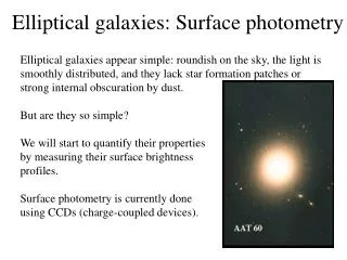
1. Elliptical galaxies: Surface photometry Elliptical galaxies appear simple: roundish on the sky, the light is smoothly distributed, and they lack star formation patches or strong internal obscuration by dust. But are they so simple? We will start to quantify their properties by measuring their surface brightness profiles. Surface photometry is currently done using CCDs (charge-coupled devices).

2. CCD detectors When a photon hits the detector, it sets free electrons, generating a current. This current is collected and amplified, and the signal produced should be linearly proportional to the number of incident photons. The surface of a CCD is divided into individual picture elements, or pixels. It is possible to do photometry (the image recorded is then a portion of the sky/star/galaxy) or spectroscopy (the light is dispersed by using a grating into its colors). There are some common problems with CCDs, which need to be taken into account in every observational program: -read-out noise (random fluctuations in the count rate: 3-10 e/pixel) -dark counts (failure to respond to currents, or electrons without an incident signal -> cooled down to 100-200 K) -Cosmic rays (energetic particles hit the detector and produce a signal which is not related to the astronomical object under study). They appear as “stars”, but if the same portion of the sky is imaged more than once, it’s unlikely a cosmic-ray will fall in the same pixel. Hence they can be corrected for.

3. Astronomy with CCD detectors • Important steps in an observational program: • Flat-fielding: pixels do not respond uniformly. Need to measure the individual response of the pixels by “observing” a diffuse screen or black twilight sky. • Calibration: Need to observe some standard stars, of known brightness to determine how many counts correspond to a given flux or magnitude. • Sky subtraction: need to subtract the contribution of the night sky, since quite often astronomical objects have brightnesses which are lower than 1% of the sky level. Hence need to get images of the blank (dark) sky, preferably close to the astronomical object under study.

4. CCD photometry - Background Inaccurate subtraction of the background contribution can mislead the following interpretation These inaccuracies in the measurement of the background emission have much worse consequences for the determination of colors, since here we have to subtract to derived quantities which themselves may contain errors.

5. The night sky • The brightness of the moonless sky is made up of 4 components: • Air glow: Photochemical processes in the upper atmosphere. It depends on the position on the sky. Changes by as much as 20% on timescales of tens of minutes. • Zodiacal light: Sunlight scattered off particles in the solar system. Makes the largest contribution. • Faint unresolved stars in our Galaxy. • Diffuse extragalactic light. • Relative importance of these components, and total intensity from them vary from site to site and with position in the sky.

6. Integrated magnitude Once we have corrected the data for these effects, we can integrate the surface brightness to get the total (integrated) brightness of the galaxy up to a given radius. The surface brightness of an object is independent of its distance to the Sun: I ~ f / DW (flux per unit solid angle) but both f and DW are proportional to ~ 1/r2, hence I is independent of the the distance to the source It is then customary to measure integrated magnitudes up to the radius of an isophote of a given magnitude, usually 26 mB.

7. Effect of Seeing One important aspect in the study of the surface brightness of galaxies is the characterization of their surface brightness profiles, that is the dependence of the surface brightness upon the projected distance to the center of the galaxy. However, turbulence in the upper atmosphere degrades the quality of an image since, due to changes in the refractive index, the light-rays from a point-like object that reach the detector have to travel slightly different paths, and hence arrive at slightly different places on the detector. The shape on the detector of an otherwise point-like source is called the Point Spread Function (or PSF), and depends both on the seeing of the site, and on the properties of the telescope-detector assembly.

8. Effect of Seeing - PSF The effect of the seeing is to blur an otherwise sharp image. If in absence of seeing the surface brightness of an object at a position R’ is It(R’), the measured brightness at a location R will be: Where P(d) is the PSF. In the simplest case, the PSF can be treated as a circularly symmetric Gaussian And it is possible to show that: Where I0 is the modified Bessel function of order 0.

9. Effect of Seeing – central core Since, as we shall see, at small radii the surface brightness profiles of galaxies go as R-g, with 0 < g < 1, the observed surface profiles (affected by seeing) would look like this: The upper curve is a power law with index –1 (R-1), while the lower curve is a power law with index –0.5. At small radii, R < s, the observed profiles have less light than the real profiles; this light is redistributed at large radii, R > s. transforming a power-law profile into a profile with a core (a central region with nearly constant surface brightness).

10. Isophotes Isophotes are contours of constant surface brightness. The ratio of semi-major to semi-minor axis measures how far the isophote deviates from a circle e = 1 – b/a. This allows to classify E galaxies by type En, where n = 10 (1-b/a)

11. Photometry of elliptical galaxies We can plot the surface brightness I(R) on the major axis of an image as a function of R. The following figure shows the surface brightness profile of the giant elliptical galaxy NGC 1700 plotted both vs. the projected distance to the center, R, and vs. R 1/4. The figure shows that an R 1/4profile would fit the data very well over some 2 decades in radius.

12. De Vaucouleurs profile The data can be fitted with a function which can be conveniently written as: With Re the effective radius, the numerical factor 3.33 is chosen such that for a circularly symmetric galaxy, if the above formula would be valid for all distance, then half of the total luminosity would be emitted inside a radius Re. The parameter Ie is clearly the surface brightness at R = Re, and the central brightness of the galaxy is I0 ~ 2000 Ie. In general, if the galaxy projects into an ellipse, Re = (aebe) 1/2.

13. Other common profiles Sersic law: where bn is chosen such that half the luminosity comes from R < Re. This law becomes de Vaucouleurs for n=4, and exponential for n=1. Hubble-Oemler law: with I0 the central surface brightness, and r0 the radius interior to which the surface brightness profile is approx. constant. For r0 < R < Rt the surface brightness changes as I ~ R–2. For R > Rt the surface brightness profile decays very quickly and predicts a finite total luminosity. In the limit Rt  this one reduces to the Hubble law:

14. De Vaucouleurs profile: deviations It is remarkable that such simple, 2-parameter profiles, fit the data of many ellipticals rather well. However, when these galaxies are studied in detail it is apparent that there is an individual behavior. However, it seems that deviations with respect to the de Vaucouleurs profile depend upon the total intrinsic luminosity of the galaxy. The figure below shows the example of a giant elliptical galaxy: There is an excess of brightness in the outer parts of the galaxy with respect to the standard de Vaucouleurs profile. In the case of dwarf ellipticals, the deviations occur in the opposite direction.

15. cD Galaxies Galaxies that show the deviations shown in the figure are called cD Galaxies. They are usually located at the center of clusters of galaxies, or in areas with dense population of galaxies. This excess emission indicates the presence of an extended halo. The cD halos are thought to belong to the cluster rather than to the galaxy. M87, the central cD galaxy in the clusters of galaxies inVirgo. Note the extended, low-surface brightness halo.

16. Deprojection of galaxy profiles So far we have discussed observed surface brightness profiles I(R), that is 3-dimensional distribution of light (stars) projected onto the plane of the sky. The question is whether we can, from this measured quantity, infer the real 3-D distribution of light, j(r) in a galaxy. If I(R) is circularly symmetric, we can assume that j(r) will be spherically symmetric, and from the following figure it is apparent that:

17. Deprojection: Abel integral This is an Abel integral equation for j as a function of I, and its solution is: A simple pair of formulae connected via the Abel integral, that approximately represent the profiles of some elliptical galaxies, are: The surface brightness profile is known as the modified Hubble law. Notice that: I ~ R-2, and j ~ r-3.

18. Deprojection: Non-spherical case If the surface brightness profile is not circularly symmetric, the galaxy cannot be spherically symmetric, but it can still be axisymmetric. In that case, if the observer looks along the equatorial plane of such object, it can be shown that is still possible to deproject the surface density profile and obtain the spatial profile. However, in general the line of sight will be inclined at an angle with respect to the equatorial plane of an axisymmetric galaxy. In that case it can be shown that there are infinite deprojected profiles that match an observation. It is easy to see that seen from the pole, both a sphere galaxy as well as any oblate or prolate ellipsoid will produce the same projected distribution as long as the 3-D radial profile is properly constructed.

19. Shapes of elliptical galaxies Can we learn something about the true distribution of ellipticities from the distribution of observed apparent ellipticities? Let’s assume that an elliptical galaxyis an oblate spheroid. The density r(x) can be expressed as r(m2), where: And a > b > 0. The contours of constant density are ellipsoids of m2 = constant. Note that when a < b, the galaxy is prolate. An observer looking down the z-axis will see an E0 galaxy, while when viewed at an angle, the system will look elliptical, with axis ratio q0 =b/a. How is q0 related to a and b ?

20. Shapes of E galaxies. Apparent axis ratios The observed axis ratio is q0 = A/(m a). The line of sight intersects the ellipsoid at (x0, z0) at the constant-density surface m. The segment A = C sin q, while C = z0 - x0 / tan q; and tan q = dx/dz. Differentiating d(m2 = x2/a2 + z2/b2 ) = 0, we find tan q = -z0/x0a2/b2 . Replacing, C = m2b2 /z0. Finally q0 = m b2 / (a z0) sin q, or q02 = cos2q + (b/a) 2sin2q This implies that the apparent axis ratio is always larger than the true axis ratio, a galaxy never appears more flattened than it actually is.

21. Shapes of elliptical galaxies. We can use the previous relation to find the distribution of apparent ellipticities produced by a random distribution of oblate/prolate ellipsoids. If the ellipsoids are randomly oriented wrt line-of-sight, then of the N(q) dq galaxies, a fraction sinq dq will have their axes oriented between q and q + dq. But we just expressed q0=q0(q). So the probability, P(q0|q) dq0, to observe a galaxy with true axis ratio q to have apparent axis ratio between q0 and q0 + dq0 is: P(q0|q) dq0 = sinq dq= sinq dq0/ | dq0 /dq|. If there are f(q0)dq0 galaxies with (observed) axis ratios in (q0,q0+ dq0 ), this should be equal to N(q) dq P(q0|q) dq0.

22. Shapes of elliptical galaxies. Distribution We have then that This is an integral equation for N(q), which can in principle be solved from the observed distribution of ellipticities. This is the observed distribution of apparent ellipticities, for 2135 E galaxies Conclusion: It is not possible to reproduce the observed distribution if all galaxies are either prolate or oblate axisymmetrical ellipsoids.

23. More on shapes. • The apparent shapes of small E are more elongated than for large E • On average, galaxies with M > -20, have q0 ~ 0.75. If they are oblate, this would correspond to 0.55 < q < 0.7 • Very luminous E, with M < -20, have on average q0 ~ 0.85. But since • there are so few that are spherical on the sky, it is very likely that most of these are actually triaxial.

24. Isophotes: deviations from ellipses Isophotes are not perfect ellipses. There may be an excess of light on the major axis (disky), or on the “corners” of the ellipse (boxy). The diskiness/boxiness of an isophote is measured by the difference between the real isophote and the best-fit elliptical one: d(f) = <d > + San cos nf + Sbn sin nf where the terms with n < 4 all vanish (by construction), and a4 > 0 is a disky E, while a4 < 0 corresponds to a boxy E.

25. Isophote twisting In a triaxial case, the orientation in the sky of the projected ellipses will not only depend upon the orientation of the body, but also upon the body’s axis ratio. This is best seen in the projection of the following 2-D figure: Since the ellipticity changes with radius, even if the major axis of all the ellipses have the same orientation, they appear as if they were rotated in the projected image. This is called isophote twisting. Unfortunately it is impossible, from an observation of a twisted set of isophotes, to conclude whether there is a real twist, or whether the object is triaxial.

26. Isophote twists Here is an example of twisted isophotes in a satellite galaxy of Andromeda (M31). The first, shallower, exposure shows the brightest part of the galaxy. The second, deeper, exposure shows the weaker more extended emission. A twist between both images of the same galaxy are apparent (the orientation in the sky is the same in both figures). Boxy galaxies are more likely to show isophote twists, more luminous in general, and probably triaxial. Disky E are midsize, more often oblate, and faster rotators. Some people have suggested disky E can be considered an intermediate class between the big boxy ones and the S0s.

27. Fine structure About 10 to 20% of the elliptical galaxies seem to contain sharp steps in their luminosity profiles. An example is the elliptical NGC 3923: These features are called ripples and shells. Ripples and shells have also been detected in S0 and Sa galaxies. Since in early-type galaxies they are detected because of the smooth profile of the underlying galaxy, it is not clear whether this is an universal phenomenon also present in later-type galaxies but difficult to detect there.

28. The kinematics of stars in E galaxies Stars in E galaxies do not follow ordered motions, but most of their kinetic energy is in the form of random motions. Moreover, the more luminous an E, the larger the velocity dispersion (which, as we have seen can be used to derive distances to E). To measure the orbital velocities of stars within galaxies is a difficult task. Absorption lines are used, which are the result of the light of all stars. Each star emits a spectrum which is Doppler shifted in wavelength according to its motion. This orbital motion makes the resulting spectral lines be wider than those of an individual star.

29. Spectra and motions of stars in E Let the energy received from a typical star, at rest with respect to the Observer, be F(l) Dl. If the star moves away from us with a velocity vz<< c, the light we receive at wavelength l, was emitted at l(1 - vz/c). To find the spectrum on the galaxy image, one needs to integrate over all stars along the line of sight (z-direction). If the number density of stars at position r with velocities in (vz, vz + dvz) is f(r, vz)dvz, the observed spectrum is If the distribution function for each type of star is known, and the spectra were the same for all stars, we could derive the spectrum of the galaxy. In practice, one makes a guess for the f(r, vz), which depends on a few parameters, and these are chosen to reproduce the observed spectrum.

30. Spectra and motions of stars in E A common choice is the Gaussian: where s(x,y) is the velocity dispersion of stars, while Vr(x,y) is the mean radial velocity at that position.

31. Scaling relations for E galaxies We have seen before that E galaxies follow the Faber-Jackson relation which can be used to derive distance to a galaxy. Note that this relation implies that more luminous galaxies have larger velocity dispersions (the typical range is from 50 km/s to 500 km/s for the brightest Es). Another scaling relation E galaxies follow is the fundamental plane. Elliptical galaxies all lie close to a plane in the 3D space defined by (velocity dispersion s, effective radius Re, surface brightness Ie). Approximately

32. The fundamental plane These plots show some of the scaling relations that E galaxies satisfy. They are all projections of the fundamental plane relation, that is shown in the last panel. They express some fundamental property of E galaxies, probably related to their formation and dynamics

33. Do Elliptical galaxies rotate? • It was initially thought that the flattened shape of some E galaxies • was due to them being fast rotators. However, observations have • shown that • Bright ellipticals (boxy) rotate very slowly, particularly in comparison • to their random motions. Their velocity ellipsoids must be anisotropic • to support their shapes. • Midsized ellipticals (disky) seem to be fast rotators

34. Stellar populations in E galaxies • It is not possible to see individual stars in galaxies beyond 10-20 Mpc. • Hence the stellar populations characteristics of E galaxies must be • derived from the integrated colors and spectra. • As we saw before, the spectra of an E galaxy resembles that of a K giant • star. • E galaxies appear generally red: • very few stars made in the last 1-2 Gyr (recall that after 1 Gyr, only • stars with masses < 2 Msun survive) • Most of the light is emitted while stars are on the giant branch • The stars in the centres of E are very metal-rich, similar to the Sun • This would seem to suggest that E galaxies are very old, however, • metallicity can also mimic age effects. Recall that metal-poor stars are • generally bluer, for the same age.

35. Stellar populations in E galaxies There is a relation between the color, and total luminosity for E galaxies. • These plots show, for galaxies in the Coma and Virgo cluster, that • Brighter galaxies are redder • Fainter systems are bluer • This could be explained if small E galaxies were younger or more metal- • poor than the large bright ones.

36. Black holes in the centres of E Some E have rising velocity dispersions as one moves closer to the centres. To keep fast moving stars within the centres, requires large masses concentrated in small regions of space, beyond what can be accounted for by the stars themselves. For example, for M32, a dwarf E satellite of M31, 2 million solar masses needed within the central 1 parsec!! The current preferred explanation is that these large masses are actually Super-massive black holes. Some believe that every galaxy harbours a SMBH. There is some evidence that the mass of the SMBH correlates with the total mass of the E galaxy.