AAVSO Citizen Sky DSLR Photometry Workshop
850 likes | 1.39k Vues
AAVSO Citizen Sky DSLR Photometry Workshop. 07 August 2009 Presented by Hopkins Phoenix Observatory. Introduction. Many people wish they could contribute something of scientific value to astronomy. The Epsilon Aurigae Project may be just the ticket.

AAVSO Citizen Sky DSLR Photometry Workshop
E N D
Presentation Transcript
AAVSO Citizen SkyDSLR PhotometryWorkshop 07 August 2009 Presented byHopkins Phoenix Observatory
Introduction Many people wish they could contribute something of scientific value to astronomy. The Epsilon Aurigae Project may be just the ticket. This talk will discuss a means to use a Digital Single Lens Reflex (DSLR) camera mounted on a tripod (no telescope needed) to do excellent V band filtered photometry on the star system from a light polluted urban backyard setting. .
Photometry To be scientifically useful, photometry must be done using standard filters that measure the brightness within a narrow band of wavelengths. The following chart is for the most popular wavelengths. While research extends into the gamma ray and radio regions, the below is where most work is done. . Photometers work in the UBV, BVRI and JH bands. 300 nano meters = 3000 Å
Photometers With proper equipment, one can do professional level photometry fairly easily. The are basically two types of photometers Single Channel Photometers. 2. CCD/DSLR Photometers Note: PEP stands for photoelectric photometry. All types of electronic photometry are PEP. .
Single ChannelPhotometers This includes Photomultiplier Tube (PMT) based photometers and PIN diode photometers, e.g., the Optec SSP-3 and SSP-4 units. For the Epsilon Aurigae Project single channel photometers are the best choice, but these may be out of reach for many. .
HPO JH Near Infrared Optec SSP-4 JH Band Photometer on 12” LX200GPS .
CCD Photometers These include astronomical CCD cameras (specifically for astronomy), modified web cams and popular Digital Single Lens Reflex CCD cameras. While monochrome cameras with standard filters are the best way to do CCD photometry, some people have used color cameras and the B, G(V) and R planes of the images to do photometry. .
HPO BVRI CCD Photometry . Modified DSI Pro with 3.3 focal reducer BVRI filter, filter wheel, and TEC/heat/sink/fan
Problems Most of the advantages of CCD photometry become disadvantages for observing epsilon Aurigae. This is because the star system is too bright and acceptable comparison stars are not in the same image. By stopping down the telescope or shortening exposures, other problems are created. .
DSLR Photometry Is it possible to use a Digital Single Lens Reflex (DSLR) color camera to do serious CCD photometry of epsilon Aurigae? .
Posibilities John Hoot presented a paper at a SAS meeting in 2007 suggesting it might be possible to use a DSLR camera for filter CCD photometry. The V band is close to the response of the Green plane of color CCDs. With proper calibration, good filter photometry should be possible. In fact it may be possible to use the Blue and Red planes also. CCD chips must use RGB filters. .
Problem Solved By using a DSLR color camera with a 50 – 100 mm lens on a tripod and splitting out the G plane, most of the problems of CCD photometry of epsilon Aurigae are solved. .
CCDs .
Color CCD Chip Typical color chip Sony ICX098BQ Note: Some chips Do not use RGB filters but Cyan, Green, Yellow and Magenta filters. .
Filter Bands Standard UBVRI filter response. Color CCD response. .
CCD Pixel Matrix . Readout of a portion of the pixel matrix. Vertical axis shows pixel ADU counts in rows 180 to 199. Horizontal axis shows ADU counts for pixels in columns 310 to 320.
Epsilon Aurigae in 3D A 3D Excel plot of the ADU counts for the pixel matrix of showing a 3 D profile of epsilon Aurigae .
Photometry Steps Single Channel 1 – Acquiring Star Data 2 – Determining Magnitudes Color CCD/DSLR 1 – Imaging Stars 2 – Split RGB Planes 3 - Acquire Star Data from the Image 4 – Determining Magnitudes .
Imaging Stars Goal: To create a computer file with the image of the star of interest and comparison star. Here is where those who have been taking pretty CCD astronomical pictures will have a large advantage. If you fall into that category you have this step mastered. In fact you should be confident with CCD photography before proceeding with CCD/DSLR photometry. .
DSI Pro with Camera Lens Test set up BVRI photometry of epsilon Aurigae with DSI Pro and 50 mm camera lens .
CCD/DSLR Camera Imaging Considerations • Star Field • Exposure/Stacking/Dark Frames • RGB Plane Splitting • Linearity problems • Under Sampling .
Star Field Make sure the program (epsilon Aurigae) and comparison (eta & zeta Aurigae) stars are all in the image. For the V band DSLR photometry of epsilon Aurigae, eta and zeta Aurigae can be used as the comparison stars. Normally lambda Aurigae is used, but it’s 5 degrees away. The further apart the program and comparison stars are the more important extinction considerations. .
Star Field Taken with DSI Pro and 50mm camera lens .
Exposure/Stacking Ideally take at least a 10 - second exposure to minimize atmospheric scintillation effects. A shorter exposure with stacked images works as well. Taking 5 – 2 second exposures and stacking them is equivalent to taking 1 – 10 second exposure. .
Dark Frames & Flat Fields Because of the short exposure (less than 1 second) dark frames are not required. While it is always a good idea to use Flat fields, for this project they are optional. .
Linearity Be aware of linearity problems. Keep peak pixel counts under 40,000 ADU. Ideally you should test your camera by using a fixed light source taking multiple images on a bench and increasing the exposure times. Then make a plot of average or peak ADU counts versus the exposure times. You should see a slanted straight line that starts to bend around 40,000 counts. Up to that point the camera is linear. .
Histogram Counts If possible monitor the peak or maximum Histogram counts for the image. Keep them well under 40,000 counts. Be sure Capella is not in the image as that will be very bright and foil the exposure. .
RGB Plane Splitting AIP4WIN and most image processing software allow easy splitting of the color image into separate R, G, and B images. More on this later. .
Under Sampling • Be aware of under sampling. • Because the individual detectors (pixels) on the CCD chip are not continuous and have gaps separating them, if light only falls on a couple of pixels, a significant amount will fall in the gaps and be lost. The more pixels covered, the less percentage of the light is lost to the cracks. • Defocusing and/or turning off tracking help spread the star image and reduce under sampling. .
Acquiring Star Data Once the image(s) has been taken (and stacked) and darks subtracted the processing starts. The goal here is to examine an image and extract total Analog to Digital Unit (ADU) counts that represent the brightness of the star or star system. This is the sum of all the ADU counts for the pixels covered by the star minus an area around the star to subtract the sky. .
Image Processing The size of the circle for the star data and a reference annulus for the sky data can be specified. .
AIP4WIN There are several software packages that allow the necessary image processing. AIP4WIN is one of the best. For under $100 it comes with a very large book (The Handbook of Astronomical Image Processing by Richard Berry and James Burnell) that is excellent for explaining much of what is going on. It’s a “must read.” .
Determining Magnitude The goal of astronomical photometry is to determine the magnitude of a star or star system as would be seen outside the Earth’s atmosphere. As we see it through the atmosphere , depending on the distance from the zenith, a constant magnitude star will be observed to be vary in brightness. .
A Review .
Brightness - Magnitude The Greeks devised the original stellar magnitude system by dividing stars into 6 groups from the brightest to the faintest they could see. The brightest were determined to be magnitude 1 and the faintest magnitude 6. A 1st magnitude star is 100 times brighter than a 6th magnitude star. . It turns out the are some stars brighter than 1st magnitude and many many stars fainter than 6th magnitude. But it was a start.
Magnitude System Magnitude = -2.5 * log10 (b) + C b is some measure of the star brightness (star measure), counts (e.g., ADU counts or number of photons) or a voltage level. C is a zero point constant dependent of the sensitivity of the equipment used. Note: That’s -2.5 not -2.512. .
Magnitudes Magnitudes as a ratio don’t need the zero point factor. Dm = -2.5 * log10 (Star 1 measure/Star 2 measure) Magnitude Difference (Dm) m = -2.5 * log10 (Star 1 measure/0 Mag Star measure) m is the measured (raw or instrumental) magnitude not the final magnitude Problem: Zero magnitude stars are rare. .
V Magnitude Equation Mv = -2.5 * log10 (SM) + e * (B-V) – X * k’v + Zpv • The equation for calculating the magnitude can be considered in several phases. • Raw or instrumental magnitude calculation. • Zero Point factor. • Extinction factor. • Color Transformation factor. • Differential Magnitude. .
Zero Point Zero points calibrate the sensitivity of the equipment. A 16” telescope will have a very different zero point than an 8” scope. .
Zero Point FactorPhase 1 m = -2.5 log10 (SM) + Zp m = raw magnitude SM= Star Measure (ADU counts) Zp = Zero Point .
Extinction Extinction is the attenuation of light due to the Earth’s atmosphere. .
Extinction Factor Stars at zenith have an Air Mass (X) = 1 and least extinction. Extinction goes up exponentially the closer to the horizon the star is. Extinction is higher at shorter wavelengths. .
Extinction Coefficient(V Band)Phase 2 k’v is a V band extinction coefficient and varies nightly. Ideally it should be determined each observation night. The extinction is the air mass (X) times the extinction coefficient k’v. [X * k’v] . mv = -2.5 log10 (SMv) – X * k’v + Zpv
Air Mass Air Mass (X) is 1.00 at the zenith and increases fast closer to the horizon. X= secZ (1- 0.0012 * (sec2Z - 1) X= secZ – 0.0018167 * (secZ -1) - 0.002875 * (secZ - 1)2 - 0.0008083 * (secZ - 1)3 secZ= (sinLat * sind + cosLAT * cosd * cosHA)-1 Z= angular distance of the star from zenith Lat= observation latitude d= star’s declination HA= star’s Hour Angle .
Color Transformation Color transformation coefficients correct for different wavelength sensitivity of the system, mainly the detector and filters. .
Color Transformation(V Band)Phase 3 For V band data the color transformation coefficient is epsilon (e) and is multiplied by the color index of the star (B-V). The closer to zero e is the better. [e * (B-V)] Mv= extra-atmospheric star V band magnitude . Mv = -2.5 log10 (SM) + e * (B-V) - X*k’v + Zpv
Differential Photometry The most accurate photometry is differential photometry. Here the difference between the star of interest (program star) and a comparison star of similar color (B-V) is measured. The comparison star should be a non-variable with known magnitudes and close in brightness to the program star. The results are then normalized to the comparison star. .
Sample Calculation DMv= Differential Magnitude = Mvp – Mvc e.g., DMv= 3.011 – 3.213 DMv= - 0. 202 Mvp and Mvc are the program and comparison star reduced magnitudes respectively. If comparison star has a listed magnitude of Mvc= 3.200 Mvp = DM + Mvc = (-0.202) + 3.200 = 2.998 Mvp = 2.998 The program star’s final V magnitude. .