Logistic Regression Example Using Horseshoe Crab Data
150 likes | 210 Vues
Study on nesting horseshoe crabs focusing on predicting satellite presence using carapace width. Analysis, output, and diagnostics shown.

Logistic Regression Example Using Horseshoe Crab Data
E N D
Presentation Transcript
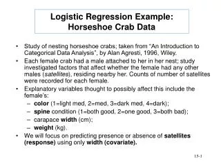
Logistic Regression Example:Horseshoe Crab Data • Study of nesting horseshoe crabs; taken from “An Introduction to Categorical Data Analysis”, by Alan Agresti, 1996, Wiley. • Each female crab had a male attached to her in her nest; study investigated factors that affect whether the female had any other males (satellites), residing nearby her. Counts of number of satellites were recorded for each female. • Explanatory variables thought to possibly affect this include the female’s: • color (1=light med, 2=med, 3=dark med, 4=dark); • spine condition (1=both good, 2=one good, 3=both bad); • carapace width (cm); • weight (kg). • We will focus on predicting presence or absence of satellites (response) using only width (covariate).
Data andsoftware code (SAS, SPSS, and R) available on Agresti’s website:http://www.stat.ufl.edu/~aa/cda/software.html
Fit model, get influence diagnostic graphs, and goodness of fit measures Note: MTB calls categorical variables factors. In Graphs, select these influence measures In Results, select maximum number of items to display
Output: Fitted Model Binary Logistic Regression: satell versus width Link Function: Logit Response Information Variable Value Count satell 1 111 (Event) 0 62 Total 173 Logistic Regression Table Odds 95% CI Predictor Coef SE Coef Z P Ratio Lower Upper Constant -12.3508 2.62873 -4.70 0.000 width 0.497231 0.101736 4.89 0.000 1.64 1.35 2.01 Log-Likelihood = -97.226 Test that all slopes are zero: G = 31.306, DF = 1, P-Value = 0.000 The odds of a crab having a satellite are 1.64 times the odds for crabs that are 1 cm shorter in width (odds increase by 64% per unit increase in width). Width is a significant predictor of incidence of satellites, as compared to just using the mean sample proportion, 111/173.
More on the Fitted Model At the mean width of x=26.3, the predicted prob of a satellite is 0.674, which corresponds to an odds of 0.674/(1-0.674)=2.07. At width of x=26.3+1=27.3, the predicted prob of a satellite is 0.773, which corresponds to an odds of 0.773/(1-0.773)=3.40. But this is an odds increase of 64%, i.e. 3.40=2.07(1.64).
Output: Goodness-Of-Fit Goodness-of-Fit Tests Method Chi-Square DF P Pearson 55.1779 64 0.776 Deviance 69.7260 64 0.291 Hosmer-Lemeshow 3.5615 8 0.894 Brown: General Alternative 1.1162 2 0.572 Symmetric Alternative 1.1160 1 0.291 Table of Observed and Expected Frequencies: (See Hosmer-Lemeshow Test for the Pearson Chi-Square Statistic) Group Value 1 2 3 4 5 6 7 8 9 10 Total 1 Obs 5 8 11 8 15 12 14 16 16 6 111 Exp 5.4 7.6 8.6 9.9 15.4 12.9 13.3 16.8 15.3 5.7 0 Obs 14 10 6 9 9 6 3 4 1 0 62 Exp 13.6 10.4 8.4 7.1 8.6 5.1 3.7 3.2 1.7 0.3 Total 19 18 17 17 24 18 17 20 17 6 173 Model passes all GOF tests
Output: Predictive Ability Measures of Association: (Between the Response Variable and Predicted Probabilities) Pairs Number Percent Summary Measures Concordant 5059 73.5 Somers' D 0.48 Discordant 1722 25.0 Goodman-Kruskal Gamma 0.49 Ties 101 1.5 Kendall's Tau-a 0.22 Total 6882 100.0 Use % concordant and discordant to compare the model to alternative models with different predictors and alternative link functions. The Summary Measuresattempt tosummarize the concordant and discordant information. These measures vary between -1 and 1, with larger values denoting greater predictive/explanatory capability, and are the logistic regression equivalent of correlation between X and Y.
Output: Diagnostic Plots A few obs are influential (leverage plot) and poorly fit (probability plot), esp. case #22 (Delta Chi-Square=5.86). Delta values in excess of 3.8 are deemed too high.
Logistic Regression in SAS proc logistic; model satell = width; Logistic Regression in SPSS ANALYZE > REGRESSION > BINARY LOGISTIC In LOGISTIC REGRESSION dialog box enter: • response: satell • covariate: width
Poisson regression with log link (in R) family=binomial for logistic reg. glm(formula = satellites ~ width, family = poisson(link = log), data = crabs) Deviance Residuals: Min 1Q Median 3Q Max -2.8526 -1.9884 -0.4933 1.0970 4.9221 Coefficients: Estimate Std. Error z value Pr(>|z|) (Intercept) -3.30476 0.54224 -6.095 1.10e-09 *** width 0.16405 0.01997 8.216 < 2e-16 *** (Dispersion parameter for poisson family taken to be 1) Null deviance: 632.79 on 172 degrees of freedom Residual deviance: 567.88 on 171 degrees of freedom AIC: 927.18 LRT for comparing model with and without width is: 632.8-567.9=64.9 on 1 df (sig.) Fitted model: log(μ) = -3.305 + 0.164 Width
Poisson regression with identity link (in R) glm(formula = satellites ~ width, family = poisson(link = identity), data = crabs, start = coef(log.fit)) Deviance Residuals: Min 1Q Median 3Q Max -2.9113 -1.9598 -0.5405 1.0406 4.7988 Coefficients: Estimate Std. Error z value Pr(>|z|) (Intercept) -11.52547 0.67767 -17.01 <2e-16 *** width 0.54925 0.02968 18.50 <2e-16 *** (Dispersion parameter for poisson family taken to be 1) Null deviance: 632.79 on 172 degrees of freedom Residual deviance: 557.71 on 171 degrees of freedom AIC: 917.01 Fitted model: μ = -11.525 + 0.549 Width
Comparison of fitted lines for log vs. identity links Identity link is a little better. (Verified by AIC.) Note: cannot use LRT for this, must use AIC.