Download
1 / 43
440 likes | 741 Vues
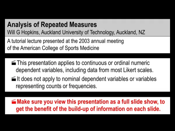
Analysis of Repeated Measures Will G Hopkins, Auckland University of Technology, Auckland, NZ. A tutorial lecture presented at the 2003 annual meeting of the American College of Sports Medicine.

E N D
Analysis of RepeatedMeasuresWill G Hopkins, Auckland University of Technology, Auckland, NZ A tutorial lecture presented at the 2003 annual meetingof the American College of Sports Medicine • This presentation applies to continuous or ordinal numeric dependent variables, including data from most Likert scales. • It does not apply to nominal dependent variables or variables representing counts or frequencies. • Make sure you view this presentation as a full slide show, to get the benefit of the build-up of information on each slide.
OVERVIEW Basics • What change has occurred in response to a treatment/intervention? • Analysis by ANOVA, within-subject modeling, mixed modeling. • Fixed and random effects; individual responses and asphericity. Accounting for Individual Responses • What is the effect of subject characteristics on the change? Analyzing for Patterns of Responses • What is the treatment's effect on trends in repeated sets of trials? Analyzing for Mechanisms • How much of the change was due to a change in whatever?
Basics What change has occurred in response to a treatment or intervention?
Period oftreatment exptal Data are means and standard deviations pre mid post control Trial or Time • Within-subjects factor • Same subjects on each level Group • Between-subjects factor • Different subjects on each level Basics: Interventions • A repeated measure is a variable measured two or more times, usually before, during and/or after an intervention or treatment. Y • Dependent variable • Repeated measure • Analysis by ANOVA, t statistics and within-subject modeling, and mixed modeling.
Measure = "Y"within-subjects factor = "Trial" Girl Group Ypre Ymid Ypost Ann exptal 58 62 68 Bev exptal 45 . 57 Lyn control 39 42 40 May control 44 45 42 Missing value means loss of subject. Basics: Analysis by ANOVA • Data are in the form ofone row per subject: • Select columns to definea within-subjects factor. • If there is no control group, use a 1-way repeated-measures ANOVA • The 1 way is Trial: • "(How) does Trial affect Y?" • With a control group, use a 2-way repeated-measures ANOVA. • The 2 ways are Group and Trial. • You investigate the interaction GroupTrial: • "(How) does Trial affect Y differently in the different groups?"
Ypost-Ypre Girl Group Ypre Ymid Ypost 10 Ann exptal 58 62 68 Bev exptal 45 . 57 12 Lyn control 39 42 40 1 Missing value does not affect post – pre changes May control 44 45 42 -2 Basics: Analysis by t Statistics and Within-Subject Modeling • If there is no control group, use a paired t statistic to investigate changes between interesting measurements. • With a control group, calculate change scores and use the unpaired t statistic to investigate the difference in the changes. • Use un/paired t statistics for other interesting combinations of repeated measurements. I call it within-subject modeling. • Example: time course of an effect…
Missing valueno problem. Basics: More Within-Subject Modeling Ann • To quantify a time course: • fit lines or curves to each subject's points; • predict interesting things for each subject; • analyze with un/paired t statistic. • Method #1. Fit lines Y= a + b.T • At Time 0 and 3, Y = a and a+3b. • Change in Y = b per week. • Method #2. Fit quadratics Y= a + b.T + c.T2 • At Time 0 and 3, Y = a and a+3b+9c. • Change in Y = 3b+9c over 3 weeks. • Maximum occurs at Time = -b/(2a). • Method #3. Fit exponentials Y= a + b.eT/c • Needs non-linear curve fitting to estimatetime constant c. Bev Lyn Y May 3 1 2 0 Time (wk)
Girl Group Trial Y Ann exptal pre 58 Ann exptal mid 62 Ann exptal post 68 Bev exptal pre 45 Bev exptal mid . Bev exptal post 57 Lyn control pre 39 Lyn control mid 42 Missing value means loss of only one trial for the subject. Basics: Analysis by Mixed Modeling • Data are in the form of one row per subject per trial: • Analysis is via maximizing likelihood of observed valuesrather than ANOVA's approachof minimizing error variance. • You investigate fixed effects: • Trial, if there's only one group. • GroupTrial, if there's morethan one group. • You also specify and estimate random effects. • "Mixed" = fixed + random. • Some mixed models are also known as hierarchical models.
Basics: Fixed Effects • Fixed effects are differences or changes in the dependent variable that you attribute to a predictor (independent) variable. • They are usually the focus of our research. • Their value is the same (fixed) for everyone in a group. • They have magnitudes represented by differences or changesin means. • Example of difference in means: • girls' performance = 48 • boys' performance = 56 • so effect of sex (maleness) on performance = 56 – 48 = 8. • Example of change in a mean: • girls' performance in pretest = 48 • girls' performance after a steroid = 56 • so effect of the steroid on girls' performance = 56 – 48 = 8.
Basics: Random Effects • Random effects have values that vary randomly within and/or between individuals. • They provide confidence limits or p values for the fixed effects. • They provide other valuable information usually overlooked. • They are mostly hidden in ANOVA, are accessible in t tests, and are up front in mixed modeling. • They are the key to understanding repeated measures. • They have magnitudes represented by standard deviations (SD). • Examples of between-subject SD or random effects: • Variation in ability: SD of girls' performance (Y) = 9.2 • Individual responses: SD of effect of a steroid on Y = 5.0, so you can say the effect of the steroid is 8.0 ± 5.0 (mean ± SD). • Example of a within-subject SD or random effect: • Error of measurement: SD of any girl's Y in repeated tests = 2.0
A girl's true performance (not observed) A girl's observed performance… in Trial #1 in Trial #2 48.3 + +7.4 =55.7 55.7 + +2.1 =57.8 55.7 + -1.3 =54.4 SD = 9.2 SD = 2.0 Girls Trials Basics: The "Hats" Metaphor for Random Effects • When you measure something, it's like adding together numbers drawn from several hats. • Each hat holds a zillion pieces of paper, each with a number. • The numbers are normally distributed with mean = 0, SD = ?? • Example: measure a girl's performance several times. Suppose true mean performance of all girls = 48.3 • The random effects in SAS are Girl and GirlTrial (= the residuals).
Performance in Trial #1 Performance in Trial #2 + Ann 55.7 + +2.1 =57.8 -1.3 55.7 + =62.4 8.0 + Bev 48.4 + -3.1 =45.3 48.4 + +0.7 =57.1 8.0 SD = 2.0 Trials + Cas 65.2 + -2.8 =62.4 65.2 + -1.4 =71.8 8.0 + Deb 40.7 + +0.5 =41.2 40.7 + +2.8 =51.5 8.0 SD = 2.0 Trials SD = 2.0 Trials • These are all we can observe. SD = 2.0 Trials Basics: Hats plus a Fixed Effect • Example: give steroid with a fixed effect of 8.0 between Trials #1 and #2, and measure several girls. • Subject hat not shown. • The stats program uses them to estimate the fixed and random effects.
Performance in Trial #1 Performance in Trial #2 + +5.2 + Ann 55.7 + +2.1 =57.8 55.7 + -1.3 =67.6 8.0 + -0.5 + Bev 48.4 + -3.1 =45.3 48.4 + +0.7 =56.6 8.0 + +6.2 + Cas 65.2 + -2.8 =62.4 65.2 + -1.4 =78.0 8.0 SD = 2.0 SD = 5.0 Individ Trials Responses + -2.7 + Deb 40.7 + +0.5 =41.2 40.7 + +2.8 =48.8 8.0 SD = 2.0 SD = 5.0 Individ Trials Responses SD = 2.0 SD = 5.0 Individ Trials Responses SD = 2.0 SD = 5.0 Individ Trials Responses Basics: A Hat for Individual Responses • Example: different responses to the steroid. • To estimate the SD for individual responses, you need a control group (see later) or an extra trial for the treatment group.
Basics: Individual Responses and Asphericity • It's important to quantify individual responses, but… • More importantly, they are the most frequent reason for the asphericity type of non-uniform error in repeated measures. • You must somehow eliminate non-uniformity of error to get trustworthy confidence limits or p values. • Here's the deal on asphericity. • Conventional ANOVA is based on the assumption that there is only one random-effects hat, error of measurement. • We can use ANOVA for repeated measures by turning the subjects random effect into a subjects fixed effect. • But it doesn't work properly when there is asphericity: that is,more than one source of error, such as individual responses. • There are four approaches to the asphericity problem.
Basics: Dealing with Asphericity in Repeated Measures • Four approaches: • MANOVA (multivariate ANOVA) • (Univariate) ANOVA with adjustment for asphericity • Within-subject modeling with the unequal-variances t statistic • Mixed modeling • I base my assessment of these approaches mainly on my experience with the Statistical Analysis System (SAS). • Other stats programs may produce different output.
Basics: MANOVA/adjusted ANOVA for Asphericity (NOT!) • Both these approaches involve different assumptions about the relationship between the repeated measurements. • They produce an overall p value for each fixed effect. • Incredibly, the p value is too small if sample size and individual responses differ between groups. • Adjusted ANOVA (Greenhouse-Geisser or Huynh-Feldt) is worse than MANOVA. • Subjects with any missing value are first deleted. • So there is needless loss of power, if the missing value is for a minor repeated measurement (e.g., post2). • In the old-fashioned approach, you are allowed to "test for where the difference is" only if the overall p<0.05. • So there is further loss of power, because you could fail to detect an effect on the overall p or the subsequent test.
Basics: More on MANOVA/adjusted ANOVA • The overall p value is OK when the extra random effects are the same in both groups, even when sample sizes differ. • Example: two repeated-measures factors; for example, several measurements on one day repeated at monthly intervals. • The program then does p values for the requested contrasts (differences in the changes; e.g., post – pre for exptal – control). • These comparisons are simply equal-variance t tests. • So the p values are too small if sample size and individual responses differ between groups. • There is no adjustment other than Bonferroni for inflation of Type I error for contrasts involving repeated measures. • Good! But researchers still dial up Tukey or other adjustments and think that the resulting p values are adjusted. They're not. • In summary: avoid MANOVA and adjusted ANOVA.
+ + = 33 Y exptal Trials Trials Trials Trials + = 8 control SD2 = 4 SD2 = 4 SD2 = 4 SD2 = 4 pre post Randomeffects: Individ Responses Individ SD2 = 25 Trials Responses SD = 2.0 SD = 5.0 Basics: Unequal-Variances t Statistic Deals with Asphericity • Example: controlled trial of effect of the steroid on performance. Variance of post–pre change scores: • Big differences in variances. • So use unequal-variances t statistic to analyze changes. • Bonus: estimate of individual responses as an SD =(SDChgExpt2– SDChgCont2)
Basics: Summary of t Statistic for Repeated Measures • Advantages • It works! • It's robust to gross departures from non-normality, provided sample size is reasonable. • 10 in each group is forgiving, 20 is very forgiving. • Missing values are not a problem. • Because you analyze separately the changes of interest. • Students can do most analyses with Excel spreadsheets. • Include my spreadsheet for confidence limits and clinical/practical/mechanistic probabilities. • You can include covariates by moving to simple ANOVAs or ANCOVAs of the change scores. • Example: how does age modify the effect of the steroid on performance? (See later.) But…
Basics: More on t Statistic for Repeated Measures • Disadvantages • ANOVAs or ANCOVAs of the change scores aren't strictly applicable, if variances of the change scores differ markedly. • You can't easily get confidence limits for the SD representing individual responses. • That is, I don't have a formula or spreadsheet yet. • There's always bootstrapping, but it's hard work. • The disdain of editors and peer reviewers, most of whom think state of the art is repeated-measures ANOVA with post-hoc tests controlled for inflation of Type I error. • In conclusion, I recommend within-subject modeling using unequal-variances t statistic for analysis of straightforward data. • Otherwise use mixed modeling…
Basics: Mixed Modeling for Asphericity • You take account of potential sources of asphericity by including them as random effects. • Advantages • It works! • Impresses editors and peer reviewers. • Confidence limits for everything. • Complex fixed-effects models are relatively easy: • individual responses, patterns of responses, mechanisms • Disadvantages • Not available in all stats programs. • Takes time and effort to understand and use. • The documentation is usually impenetrable. • Sample size for robustness to non-normality not yet known.
Accounting forIndividual Responses What is the effect of subject characteristics on the change?
boys girls Y Data arevalues forindividuals pre mid post pre mid post Trial Individual Responses: and Subject Characteristics • Subjects differ in their response to a treatment… …due to subject characteristics interacting with the treatment. • It's important to measure and analyze their effect on the treatment. • Using value of Trialpre as a characteristic needs special approach to avoid artifactual regression to the mean. See newstats.org. • Use mixed modeling, ANOVA, or within-subject modeling.
Individual Responses: byMixed Modeling • You include subject characteristics as covariates in the fixed-effects model. • The SD representing individual responses will diminish and represent individual responses not accounted for by the covariate. • The precision of the estimates of the fixed effects usually improves, because you are accounting for otherwise random error. • Covariates can be nominal (e.g., sex) or numeric (e.g., age). • Example: how does sex affect the outcome? • First, you can avoid covariates by analyzing the sexes separately. • Effect on females = 8.8 units; effect on males = 4.7 units. • Effect on females – males = 8.8 – 4.7 = 4.1 units. • You can generate confidence limits for the 4.1 "manually", by combining confidence limits of the effect for each sex. • Include individual responses for each sex: 8.8 ± 5.2; 4.7 ± 2.5.
Individual Responses: More Mixed Modeling • The full fixed-effects model is Y GroupTrial SexGroupTrial. • The term SexGroupTrial yields the female-male difference of 4.1 units (90% confidence limits 1.5 to 6.7, say). • The overall effect of the treatment (from GroupTrial) is for an average of equal numbers of females and males. • Try including random effects for individual responses in males and females. • Example: how does age affect the outcome? • Either: convert age into age groups and analyze like sex. • Or: if the effect of age is linear, use it as a numeric covariate. • AgeGroupTrial provides the outcome as effect per year: 1.3 units.y-1 (90% confidence limits -0.2 to 2.8). • Note that the overall effect of the treatment is for subjects with the average age.
Individual Responses: by Repeated-Measures ANOVA • It is possible in principle to include a subject characteristic as a covariate in a repeated-measures ANOVA. • But SPSS (Version 10) provides only the p value for the interaction. Incredibly, it does not provide magnitudes of the effect. • If a covariate accounts for some or all of the individual responses, the problem of asphericity will diminish or disappear. • I don't know whether it's possible to extract the SD representing individual responses from a repeated-measures ANOVA, with or without a covariate.
Ypost-Ypre Kid Sex Age Group Ypre Ymid Ypost Ann F 23 exptal 58 62 68 10 4 Ben M 19 exptal 64 67 68 Lyn F 19 control 39 42 40 1 Merv M 19 control 59 60 57 -1 Individual Responses: byWithin-Subject Modeling • Calculate the most interesting change scores or other within-subject parameters: • If no control group, analyze effect of subject characteristics on change score with unpaired t, regression, or 1-way ANOVA. • With a control group, analyze with 2-way ANOVA. • As before, a characteristic that accounts partially for individual responses will reduce the problem of asphericity.
Analyzing for Patterns of Responses What is the effect of a treatment on trends within repeated sets of trials?
1 2 Bout 3 exptal 4 Y Standard deviations: Between Subjects within Bout control Within Subject between Trials pre mid post Within Subject within Trial Trial Patterns of Responses: Bouts within Trials • Typical example: several bouts for each of several trials. • We want to estimate the overall increase in Y in the exptal group in the mid and post trials, and… • …the greater decline in Y in the exptal group within the mid and post trials (representing, for example, increased fatigue). • Use mixed modeling, ANOVA, or within-subject modeling.
Patterns of Responses: byMixed Modeling and ANOVA • With mixed modeling, Bout is simply another (within-subject) fixed effect you add to the model. • The model is Y Trial Bout TrialBout. • Bout can be nominal or numeric. • If numeric, Bout specifies the slope of a line, and TrialBout specifies a different slope for each level of Trial. • Add BoutBout(Trial) to the model for quadratic(s). • Elegant and easy, when you know how. • With ANOVA, you have to specify Bout as a nominal effect and try to take into account within-subject errors using adjustments for asphericity. • Specifying a quadratic or higher-order polynomial Bout effect is possible but difficult (for me, anyway). • Within-subject modeling is much easier…
Subject: JC Y pre mid post Trial Patterns of Responses: byWithin-Subject Modeling • The trick is to convert the multiple Bout measurements into a single value for each subject, then analyze those values. • In the example, derive the Bout mean and slope(or any other parameters) within each trial for each subject. • Derive the change in meanand the change in slopebetween pre and post(or any other Trials) for each subject. • For the changes in the mean, do an unpaired t test between the exptal and control groups. Ditto for the changes in the slope. • Simple, robust, highly recommended!
Analyzing for Mechanisms How much of the change was due to a change in whatever?
Mechanism variable Dependent variable exptal exptal control control pre mid post pre mid post Trial Analyzing for Mechanisms • Mechanism variable = something in the causal path between the treatment and the dependent variable. • Necessary but not sufficient that it "tracks" the dependent. • Important for PhD projects or to publish in high-impact journals. • It can put limits on a placebo effect, if it's not placebo affected. • Can't use ANOVA; can use graphs and mixed modeling.
Measure = "Y"within-subjects factor = "Trial" Mechanism variable(within-subjects covariate) Girl Group Ypre Ymid Ypost Xpre Xmid Xpost Ann exptal 58 62 68 8.4 8.7 9.1 Bev exptal 45 . 57 9.0 . 9.7 Lyn control 39 42 40 7.9 7.7 7.8 May control 44 45 42 7.1 7.1 7.2 Mechanisms: Why not ANOVA? • For ANOVA, data have to be one row per subject: • You can't use ANOVA, because it doesn't allow you to match up trials for the dependent and covariate.
Change scorefor dependent Ypost-Ypre Xpost-Xpre Girl Group Ypre Ymid Ypost Xpre Xmid Xpost Ann exptal 58 62 68 8.4 8.7 9.1 10 1.5 Bev exptal 45 . 57 9.0 . 9.7 12 0.7 Lyn control 39 42 40 7.9 7.7 7.8 1 -0.1 May control 44 45 42 7.1 7.1 7.2 -2 0.1 Change scorefor covariate Mechanisms: Analysis Using Graphs • Choose the most interesting change scoresfor the dependent and covariate: • Then plot the change scores…
1. Large individual responses… …tracked by mechanism variable… …even in the control group. exptal Ypost - Ypre 0 control 0 Xpost - Xpre Mechanisms: MoreAnalysis Using Graphs • Three possible outcomes with a real mechanism variable: • The covariate is an excellent candidate for a mechanism variable.
Ypost - Ypre 0 0 Xpost - Xpre Mechanisms: MoreAnalysis Using Graphs • Three possible outcomes with a real mechanism variable: 2. Apparently poor tracking of individual responses… … but it could be due to noise in either variable. • The covariate could still be a mechanism variable.
3. Little or no individual responses… …but mechanism variable tracks mean response. Ypost - Ypre 0 0 Xpost - Xpre Mechanisms: MoreAnalysis Using Graphs • Three possible outcomes with a real mechanism variable: • The covariate is a good candidate for a mechanism variable.
Ypost – Ypre 0 0 0 Xpost – Xpre Mechanisms: Graphical Analysis – how NOT to • Relationship between change scores is often misinterpreted. • "The correlation between change scores for X and Y is trivial. • Therefore X is not the mechanism." • "Overall, changes in X track changes in Y well, but… • Noise may have obscured tracking of any individual responses. • Therefore X could be a mechanism variable."
Mechanism variable(within-subjects covariate) Girl Group Trial Y X Ann exptal pre 58 8.4 Ann exptal mid 62 8.7 9.1 Ann exptal post 68 Bev exptal pre 39 9.0 • No problem with aligning trials for the dependent and covariate. Mechanisms: Quantitative Analysis by Mixed Modeling - 1 • Need to quantify the role of the mechanism variable, with confidence limits. • I have devised a method using mixed modeling. • Data format isone row per trial:
Mechanisms: MoreQuantitative Analysis by Mixed Modeling • Run the usual fixed-effects model to get the effect of the treatment. • Example: 4.6 units (90% likely limits, 2.1 to 7.1 units). • Then include a putative mechanism variable in the model. • The model is then effectively a multiple linear regression, so… • You get the effect of the treatment with the mechanism variable held constant… • …which means the same as theeffect of the treatment not explained by the putative mechanism variable. • Example: it drops to 2.5 units (90% likely limits, -1.0 to 7.0 units). • So the mechanism accounts for 4.6 - 2.5 = 2.1 units. • If the experiment was not blind, the real effect is >2.1 units… • …and the placebo effect is <2.5 units... • …provided the mechanism variable itself is not placebo affectible!
Summary Basics • Use the unequal-variance t statistic and within-subject modeling for straightforward models. • Repeated-measures ANOVA may not cope with non-uniform error. • Mixed modeling is best for fixed and random effects. Accounting for Individual Responses • Use within-subject modeling or mixed modeling. Analyzing for Patterns of Responses • Use within-subject modeling or mixed modeling. Analyzing for Mechanisms • Interpret graphs of change scores properly. • Use mixed modeling to get estimates of the contribution of a mechanism variable.
This presentation was downloaded from: A New View of Statistics newstats.org SUMMARIZING DATA GENERALIZING TO A POPULATION Simple & Effect Statistics Precision of Measurement Confidence Limits Statistical Models Dimension Reduction Sample-Size Estimation