CS 6234 Advanced Algorithms: Splay Trees, Fibonacci Heaps, Persistent Data Structures

1. CS 6234 Advanced Algorithms:Splay Trees, Fibonacci Heaps, Persistent Data Structures

2. Splay Trees Muthu Kumar C., XieShudong Fibonacci Heaps Agus Pratondo, AleksanrFarseev Persistent Data Structures: Li Furong, Song Chonggang Summary Hong Hande

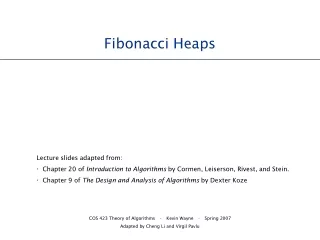
3. SOURCES: Splay Trees Base slides from: David Kaplan, Dept of Computer Science & Engineering, Autumn 2001 CS UMD Lecture 10 Splay Tree UC Berkeley 61B Lecture 34 Splay Tree • Fibonacci Heap • Lecture slides adapted from: • Chapter 20 of Introduction to Algorithms by Cormen, Leiserson, Rivest, and Stein. • Chapter 9 of The Design and Analysis of Algorithms by Dexter Kozen. • Persistent Data Structure • Some of the slides are adapted from: • http://electures.informatik.uni-freiburg.de

4. Pre-knowledge: Amortized Cost Analysis • Amortized Analysis • Upper bound, for example, O(log n) • Overall cost of a arbitrary sequences • Picking a good “credit” or “potential” function • Potential Function: a function that maps a data structure onto a real valued, nonnegative “potential” • High potential state is volatile, built on cheap operation • Low potential means the cost is equal to the amount allocated to it Amortized Time = sum of actual time + potential change

5. Splay Tree Muthu Kumar C. Xie Shudong

6. Background Balanced Binary Search Trees Unbalanced binary search tree Balanced binary search tree Zig x y y x C A B C A B Balancing by rotations Rotations preserve the BST property

7. Motivation for Splay Trees Problems with AVL Trees • Extra storage/complexity for height fields • Ugly delete code Solution: Splay trees (Sleator and Tarjan in 1985) • Go for a tradeoff by not aiming at balanced trees always. • Splay trees are self-adjusting BSTs that have the additional helpful property that more commonly accessed nodes are more quickly retrieved. • Blind adjusting version of AVL trees. • Amortized time (average over a sequence of inputs) for all operations is O(log n). • Worst case time is O(n).

8. Since you’re down there anyway, fix up a lot of deep nodes! Splay Tree Key Idea 10 17 You’re forced to make a really deep access: 5 2 9 3 Why splay? This brings the most recently accessed nodes up towards the root.

9. Splaying • Bring the node being accessed to the root of the tree, when accessing it, through one or more splay steps. • Asplay step can be: • Zig Zag • Zig-zig Zag-zag • Zig-zag Zag-zig Single rotation Double rotations

10. Splaying Cases Node being accessed (n) is: • the root • a child of the root Do single rotation: Zig or Zag pattern • has both a parent (p) and a grandparent (g) Double rotations: (i) Zig-zig or Zag-zag pattern: g  p  n is left-left or right-right (ii) Zig-zag pattern: g  p  n is left-right or right-left

11. Case 0: Access rootDo nothing (that was easy!) root root n n X Y X Y

12. Case 1: Access child of rootZig and Zag (AVL single rotations) root root p n Zig – right rotation n Z X p Zag – left rotation X Y Y Z

13. Case 1: Access child of root:Zig (AVL single rotation) - Demo Zig root p n Z X Y

14. Case 2: Access (LR, RL) grandchild:Zig-Zag (AVL double rotation) g n X p g p n W X Y Z W Y Z

15. Case 2: Access (LR, RL) grandchild:Zig-Zag (AVL double rotation) g Zig X p n W Y Z

16. Case 2: Access (LR, RL) grandchild:Zig-Zag (AVL double rotation) Zag g X n Y p Z W

17. Case 3: Access (LL, RR) grandchild:Zag-Zag (different from AVL) 1 g n 2 W p p Z X n g Y Y Z W X No more cookies! We are done showing animations.

18. Quick question In a splay operation involving several splay steps (>2), which of the 4 cases do you think would be used the most? Do nothing | Single rotation | Double rotation cases Zig x y y x C A n B C A B A B z x y D Zig-Zag z y A x C D A B B C

19. Why zag-zag splay-op is better than a sequence of zags (AVL single rotations)? 6 1 1 1 2 2 zag zags 2 3 3 ……… 3 4 4 4 6 5 Tree still unbalanced. No change in height! 5 5 6

20. Why zag-zag splay-step is better than a sequence of zags (AVL single rotations)? 1 1 1 6 2 2 2 1 3 … 3 3 3 4 5 6 2 5 5 6 4 5 4 6 4

21. Why Splaying Helps • If a node n on the access path, to a target node say x, is at depth d before splaying x, then it’s at depth <= 3+d/2 after the splay. (Proof in Goodrich and Tamassia) • Overall, nodes which are below nodes on the access path tend to move closer to the root • Splaying gets amortized to give O(log n) performance. (Maybe not now, but soon, and for the rest of the operations.)

22. Splay Operations: Find • Find the node in normal BST manner • Note that we will always splay the last node on the access path even if we don’t find the node for the key we are looking for. • Splay the node to the root • Using 3 cases of rotations we discussed earlier

23. 6 5 4 Splaying Example:using find operation 1 1 2 2 zag-zag 3 3 Find(6) 4 5 6

24. 6 5 4 … still splaying … 1 1 2 6 zag-zag 3 3 2 5 4

25. 6 1 … 6 splayed out! 1 6 zag 3 3 2 5 2 5 4 4

26. Splay Operations: Insert • Can we just do BST insert? • Yes. But we also splay the newly inserted node up to the root. • Alternatively, we can do a Split(T,x)

27. Digression: Splitting • Split(T, x) creates two BSTs L and R: • all elements of T are in either L or R (T = L  R) • all elements in L are  x • all elements in R are  x • L and R share no elements (L  R = )

28. Splitting in Splay Trees How can we split? • We can do Find(x), which will splay x to the root. • Now, what’s true about the left subtree L and right subtree R of the root? • So, we simply cut the tree at x, attach x either L or R

29. Split split(x) splay T L R OR L R L R •  x > x < x •  x

30. split(x) L R Back to Insert x L R < x > x

31. Insert Example 4 4 6 6 split(5) 1 6 1 9 1 9 9 2 2 7 4 7 7 5 2 4 6 Insert(5) 1 9 2 7

32. find(x) L R Splay Operations: Delete Do a BST style delete and splay the parent of the deleted node. Alternatively, x delete (x) L R < x > x

33. splay L R R Join Join(L, R): given two trees such that L < R, merge them Splay on the maximum element in L, then attach R L

34. find(x) L R Delete Completed x T delete x L R < x > x Join(L,R) T - x

35. Delete Example 4 6 6 1 6 1 9 1 9 find(4) 9 2 2 7 4 7 Find max 7 2 2 2 1 6 1 6 Delete(4) 9 9 Compare with BST/AVL delete on ivle 7 7

36. Splay implementation – 2 ways • Bottom-up Top Down Zig L R L R y x y x Zig y x x C C A A B y B C A B A B C Why top-down? Bottom-up splaying requires traversal from root to the node that is to be splayed, and then rotating back to the root – in other words, we make 2 tree traversals. We would like to eliminate one of these traversals.1 How? time analysis.. We may discuss on ivle. 1. http://www.csee.umbc.edu/courses/undergraduate/341/fall02/Lectures/Splay/ TopDownSplay.ppt

37. Splay Trees: Amortized Cost Analysis Amortized cost of a single splay-step Amortized cost of a splay operation: O(logn) Real cost of a sequence of m operations: O((m+n) log n)

38. Splay Trees: Amortized Cost Analysis

39. Splay Trees Amortized Cost Analysis Amortized cost of a single splay-step Lemma 1: For a splay-step operation on x that transforms the rank function r into r’, the amortized cost is: (i) ai ≤ 3(r’(x) − r(x)) + 1 if the parent of x is the root, and (ii) ai ≤ 3(r’(x) − r(x)) otherwise. Zig x y y x z x y y z Zig-Zag x

40. Splay Trees Amortized Cost Analysis Lemma 1: (i) ai ≤ 3(r’(x) − r(x)) + 1 if the parent of x is the root, and (ii) ai ≤ 3(r’(x) − r(x)) otherwise. Proof : We consider the three cases of splay-step operations (zig/zag, zigzig/zagzag, and zigzag/zagzig). Case 1 (Zig / Zag) : The operation involves exactly one rotation. Amortized cost is ai = ci + φ’ − φ x y Real cost ci = 1 y x Zig

41. Splay Trees Amortized Cost Analysis Amortized cost is ai = 1 + φ’ − φ In this case, we have r’(x)= r(y), r’(y) ≤ r’(x) and r’(x) ≥ r(x). So the amortized cost: ai = 1 + φ’ − φ = 1 + r’(x) + r’(y) − r(x) − r(y) = 1 + r’(y) − r(x) ≤ 1 + r’(x) − r(x) ≤ 1 + 3(r’(x) − r(x)) x y y x Zig

42. Splay Trees Amortized Cost Analysis Lemma 1: (i) ai ≤ 3(r’(x) − r(x)) + 1if the parent of x is the root, and (ii) ai ≤ 3(r’(x) − r(x)) otherwise. The proofs of the rest of the cases, zig-zig pattern and zig-zag/zag-zig patterns, are similar resulting in amortized cost of ai ≤ 3(r’(x) − r(x)) Zig x y y x z x y y z Zig-Zag x

43. Splay Trees Amortized Cost Analysis Amortized cost of a splay operation:O(logn) Building on Lemma 1 (amortized cost of splay step), We proceed to calculate the amortized cost of a complete splay operation. Lemma 2: The amortized cost of the splay operation on a node x in a splay tree is O(log n). Zig x y y x z x y y z Zig-Zag x

44. Splay Trees Amortized Cost Analysis Zig x y y x z x y z Zig-Zag y x

45. Splay Trees Amortized Cost Analysis Theorem: For any sequence of m operations on a splay tree containing at most n keys, the total real cost is O((m + n)log n). Proof: Let ai be the amortized cost of the i-th operation. Let ci be the real cost of the i-th operation. Let φ0 be the potential before and φm be the potential after the m operations. The total cost of m operations is: We also have φ0 − φm ≤ n log n, since r(x) ≤ log n. So we conclude: (From )

46. Range Removal [7, 14] 10 17 5 13 3 22 6 8 16 7 9 Find the maximum value within range (-inf, 7), and splay it to the root.

47. Range Removal [7, 14] 10 6 17 5 13 3 22 8 7 16 9 Find the minimum value within range (14, +inf), and splay it to the root of the right subtree.

48. Range Removal [7, 14] 6 5 16 X 10 17 3 8 13 22 [7, 14] 7 9 Cut off the link between the subtree and its parent.

49. Splay Tree Summary

50. Splay Tree Summary Can be shown that any M consecutive operations starting from an empty tree take at most O(M log(N))  All splay tree operations run in amortized O(log n) time O(N) operations can occur, but splaying makes them infrequent Implements most-recently used (MRU) logic • Splay tree structure is self-tuning