Capital Budgeting in the Chemical Industry Guest Lecture ChE 473K, Process Design and Operations

1. Capital Budgeting in the Chemical Industry Guest Lecture ChE 473K, Process Design and Operations Prof. Poehl, Spring 2014 Gerald G. McGlamery, Jr., Ph.D., P.E. Breakthrough Advisor Global Chemical Research ExxonMobil Chemical Company Baytown, Texas

2. Agenda • Review of Time Value of Money • Review of Measures of Return on Investment • Basic Concepts of Risk • Stochastic Modeling • Cash Flow Bases

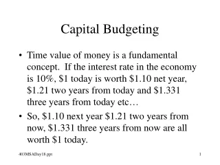
3. Review of Time Value of Money • Time Value of Money • Cost of Capital • Inflation

4. Time Value of Money The value of money decreases with time because of • inflation • uncertainty about the future, i.e. risk • the desire for liquidity

5. Sources of Capital • Debt • Equity • Common Stock • Preferred Stock • Retained Earnings

6. Cost of Capital • Cost of debt • Generally the lowest-cost source of capital because of the tax benefit. • Must be paid, however, even if the venture loses money. • Increases the risk of insolvency losses; risk premium therefore increases. • Cost of equity • Can be valued as a function of the stock dividend, the dividend growth rate, and the stock market value. • Can also be valued as a function of the risk-free return, the premium for equities over the risk free rate, and the correlation of the stock’s return with the market’s return (beta). • Companies finance capital with equity to reduce the risk of failure. • Cost of retained earnings • Treated as the equivalent of common stock. • Investors have an expectation that the retained earnings will yield the same return as the stock.

7. Inflation • Inflation is an increase in the general level of prices. • In general, the U.S. Urban Consumer Price Index (CPI) is the accepted standard for measuring inflation. • For individual goods and services, projecting future values is not the same as adjusting for inflation. • For example, $1000 will purchase more computing power in 2014, but it will purchase fewer goods and services in general than in 2013.

8. Inflation (continued) Value Adjustment • Project future values for an individual good or service in constant dollars, accounting for fundamental changes in supply and demand (including inputs). • Then, adjust for inflation to reflect the reduced buying power of money for all goods and services. • Some products might warrant no value adjustment. Actual Value or Price Inflation Present Year Next Year

9. Review of Measures of Return on Investment • Net Present Value • Internal Rate of Return • Inflating Cash Flows • Investment Hurdle Rates

10. Net Present Value The net present value (NPV) is the sum of all cash flows after discounting each cash flow for the discount rate, i. Nominal Cash Flows Net Present Value Discounted Cash Flows

11. Internal Rate of Return • The internal rate of return (IRR) is the discount rate that results in an NPV of zero. • Multiplying both sides by (1 + i)z, the IRR equation can be recast as

12. Flaws of Internal Rate of Return Project A Nominal Cash Flows IRR = 15.1 % NPV @ 5 % = $1361 NPV @ 8 % = $855 • On the basis of IRR, Project A is preferred. • On the basis of NPV @ 5 %, Project B is preferred. • On the basis of NPV @ 8 %, Project A is preferred. • IRR does not detect the sensitivity of a project to discount rate and therefore risk. • The riskier the project, the more valuable the early cash flows. • IRR does not account for differences in project life or investment magnitude. Project B Nominal Cash Flows IRR = 12.6 % NPV @ 5 % = $1437 NPV @ 8 % = $769

13. Flaws of Internal Rate of Return (continued) • Recall the second form of the IRR equation: • The IRR equation is a polynomial in (1 + i). • A polynomial will have as many real roots as it has sign changes. Nominal Cash Flows

14. Inflating Cash Flows • Inflate revenue and costs with time rather than using constant currency values. • Reasoning: • Because depreciation is not inflated, inflation cannot be added simply to constant-currency IRR. • Cost of capital has inflation built into risk-free rate.

15. Investment Hurdle Rates Companies set investment hurdle rates over the cost of capital because • deterministic methods of analysis do not account for uncertainty • resources other than cash are limited

16. Basic Concepts of Risk • Definition of Risk • Comparisons of Risk

17. Definition of Risk • Risk is characterized by the • probability of an event. • magnitude of an event. • For our purposes, we characterize risk as the probability distribution of outcomes of an event.

18. Comparisons of Risk • Project A is less risky than Projects B and C because of its small standard deviation. • Projects B and C have the potential for greater loss and greater gain than project A. • Projects B and C have equal risk, but Project B has a higher NPV at all probabilities. • Projects B and C both have significant, though not large, probabilities of losing money. • Remember, this is a cumulative distribution, so the probability shown is the probability for an NPV less than or equal to a certain value. Would you choose project A or project C?

19. Stochastic Modeling • Basis of Stochastic Modeling • Choosing Variables for Modeling • Sources of Data • Cognitive Biases • Time Correlation of a Variable • Correlating Two or More Variables • Bounded Sums

20. Basis of Stochastic Modeling • Stochastic modeling relies on repeated sampling from input variables described by probability distribution functions to generate a probability distribution function for one or more output variables. • When the sampling is random, the analysis is called Monte Carlo analysis. f(xi) The resulting distribution is frequently normal. Why?

21. Choosing Variables for Modeling • Sensitivity analysis • Input variables are systematically varied an equal amount above and below the base case to see which input variables yield the greatest changes in the output variables. • The more sensitive the model is to a variable, the more effort should go into modeling that variable. • Input variable range is important • If variable range is based on simple percentage of base value, output range will reflect only sensitivity of model • If variable range is based on statistical distribution, output range will also reflect uncertainty in input variable. • Use the fewest number of variables that will capture 80–90 % of the output variation.

22. Tornado Plots • The tornado plot is effective for ranking the effects of various inputs on an output variable. • Sensitivity of model to variable • Magnitude of uncertainty in variable • Use the tornado plot also to diagnose model errors. • Bars of zero magnitude • Bar signs that are reversed

23. Common Sense Tests In the chemical industry, economic models typically will be most sensitive to: • Product price / sales volume • Major raw material prices • Investment costs

24. Sources of Data The information you have is not the information you want. The information you want is not the information you need. The information you need is not the information you can obtain. The information you can obtain costs more than you want to pay. Most people overestimate the amount of information that is available to them. Peter Bernstein Against the Gods: The Remarkable Story of Risk In God we trust. All others must bring their data.

25. Sources of Data (continued) • The Internet • Consulting Firms • Experts, Gurus, Gray-beards, etc.

26. Example Consulting Firms • IHS Chemical • ICIS • NexantChemSystems • Platts (McGraw-Hill) • Solomon Associates • Phillip Townsend Associates (PTAI) • Argus DeWitt • TecnonOrbiChem • Chemical Data Inc. (CDI)

27. Experts, Gurus, Gray-Beards, etc. • Data on variability are rarely available in published sources, though they can be estimated from historical data. • Engineering judgment is a valid source of estimates of variability. • Be aware, however, that engineering judgment is subject to motivational and cognitive biases.

28. Cognitive Biases • Anchoring and adjustment • People frequently anchor to an initial estimate and adjust for uncertainty when assessing probability. • Availability • Information that is recent, dramatic, certified, or imaginable can increase a person’s assessment of probability. • Representativeness • Current evidence can be mistaken for long-term trends. • Implicit conditioning • People tend to make unstated assumptions when assessing probability.

29. Coping with Cognitive Bias • Motivate the expert by describing the stochastic modeling process and the use of the results. • Decompose the model to eliminate unstated assumptions. • Clearly state definitions. • What is the price of gasoline? • What is the price of unleaded regular motor gasoline, delivered to New York harbor? • Communicate using probabilities. Try to develop values for 10 %, 50 %, and 90 % cases as a minimum. • Clearly state the scenarios that yield the 10/50/90 % cases. • Verify the expert is comfortable with the result.

30. An Example of Conditioning

31. Time Correlation of a Variable Deterministic model Example: model sales volume growth of 2 %/year Each year is independent Each year is dependent on the prior year Each year is correlated with time

32. Correlating Two or More Variables — Indexing • Lacking a better correlation, some variables can be indexed to other variables: • Examples of variables that can be indexed: • Hydrogen natural gas • Oxygen industrial electricity • Nitrogen industrial electricity • Steam industrial primary energy • Freight diesel fuel

33. Correlating Two or More Variables - Regression y = ax + b • The linear regression model is actually • Linear regression estimates the coefficients describing a straight line: y = ax + b + N(0,σ) where σ is the error about the regression line. • The error is given in most regression statistics as the mean square error (MSE). The square root of the MSE is σ. • The same concept applies for non-linear regressions.

34. Bounded Sums • Bounded sums arise frequently in chemical engineering models, e.g. the sum of the selectivities must equal 1. • Varying a bounded sum randomly can violate the bound if each element is not dependent on the other. • One solution is to choose three cases of sums that would be equivalent to 10/50/90 % cases on a continuous distribution function. • The three cases can be assigned probabilities of 25/50/25 % and simulated as a discrete distribution function. • In a spreadsheet, put all three cases in an array and use the INDEX function to select the correct case.

35. Cash Flow Bases • Definitions • Marginal Cash Flows • Valuation of Chemicals • Modeling Prices and the Experience Curve • Integrated Value Chains • Supply Chain Costs • International Considerations

36. Definitions

37. Marginal Cash Flows Marginal Revenue Profit Maximized • Profits are maximized when marginal revenue equals marginal cost. • Cash flows for new investment should be based on highest cost and lowest price. • If I cannot expand and I get a higher margin sale, I would always forgo a lower margin sale. • It follows that each investment in incremental capacity becomes harder and harder to justify. Marginal Revenue and Costs Marginal Cost Sales Volume

38. Valuation Bases • Market price • Best option if available • Remember to use marginal value • Substitute or value price • Equivalent functionality or value to another product • Normalized to mass, volume, area, length, etc. • Next best disposition • Commonly found in refineries • Remember debit for replacement material • Cost of disposal

39. Correlation Between Product and Input Prices No. 2 Heating Oil vs Brent Crude • Generally a high correlation between product prices and raw materials in CPI. • Most petrochemicals highly correlated with either crude oil or natural gas. • Other energy-intensive industries (e.g. metals, transportation) correlated with energy prices. Propane vs WTI Crude

40. Price Models • Many models based on simple gross margin over raw materials. • Constant margin in currency per unit mass (e.g. USD/T). • Constant margin percentage of net raw materials. • Other model types are possible: • Smoothing • Correlative (regression) • Theoretical / explanatory (supply/demand models) • Don’t confuse prices today with long-term trends. • Transition from present prices to trend might be necessary. • New capacity usually depresses prices below trend in early years. • Add variability to near-term price trend, if not all years of project.

41. Examples of Historical Price Trends Motor Gasoline (average price), 2011USD/gal Aluminum, 1998USD/T Source: U.S. Department of Energy Source: U.S. Geological Survey Ammonia, 1998USD/T Lime, 1998USD/T Source: U.S. Geological Survey Source: U.S. Geological Survey

42. Pressures on Price • Downward trend of constant-currency prices with time is known as an experience curve. • Downward price pressures result from: • Competition • Substitution • Innovations in end-use applications • Producers always under pressure to keep up. • Learning curve • Economies of scale • Innovations in processes • Deviations from trend result from: • Changes in input (raw material, labor, capital) prices. • Changes in industry capacity utilization (supply versus demand).

43. One Formulation of the Experience Curve • Typical value-added decline for petrochemicals is 20 – 40 % per doubling of cumulative production. • Raw materials have their own experience curves. • Regional variations typically explained by exchange rates, transportation, trade barriers. Historical Prices and Costs Regression Projected Prices and Costs

44. Value Added versus Variable Margin

45. Experience Curve Implications for Capital Budgeting • Price forecasts in constant currency should assume a decline with time. • Possible forms: • Percentage price decline per year • Percentage price decline with cumulative industry production • Percentage margin decline per year • Percentage margin decline with cumulative industry production • Value-added experience curve • Experience curve effects should apply to both product prices and input prices.

46. Integrated Value Chains (the transfer price problem) A • Product B is valued at market in best case. • Frequently, B is not sold in commerce, or only a fraction of total production can be sold in commerce. • If value of B is too high, then no profit left to justify expansion of Unit 2; if too low, then no profit left to justify expansion of Unit 1. • Frequently, expansion of Units 1 and 2 not justified simultaneously. • Must pick arbitrary price marker that allows profitable return for expansion of both Units 1 and 2. 1 B 2 C

47. Integrated Value Chains (economic scope) A • An economy of scope occurs when a firm can produce B and C cheaper together than can separate companies. • If NPV of unit 1 is negative, but NPV of unit 2 and sum of both is positive, many firms frequently invest. • Investment is only justified, however, if economy of scope is possible. • If economy of scope is not possible, then firm might align with partner with lower cost of capital or existing supplier, since market might be oversupplied. 1 B 2 C

48. Supply Chain Costs • Operating Costs • Freight costs (inbound and outbound) • Freight mode changes • Storage rental • Working Capital • Plant and forward inventories • Accounts payable/receivable

49. International Considerations • Currency • Tax rules • Rates • Depreciation • Investment allowances and credits • Repatriation of funds and transfer pricing • Ownership • Profit sharing • Cost of capital • Trade costs • Tariffs, duties, drawbacks • Non-financial barriers • Frictional costs, e.g. traders, freight forwarders

50. Spreadsheet Economic Models • Flexibility is the key to a good model. • Avoid hard-coding data. • Do unit, molecular weight, and density conversions in the spreadsheet. • Use the workbook concept to organize the model in modules that are easy to update. Separate inputs, outputs, and calculations on separate pages. • Take advantage of built-in functions. • Note that Excel’s NPV function discounts the first-period cash flow. • Use the MIN or MAX functions to bound calculations. • Be careful with linking spreadsheets. • Values have a habit of changing when you least expect it. • Document everything!