We use Numerical continuation Bifurcation theory with symmetries

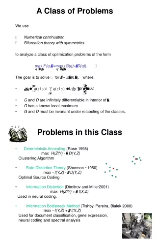
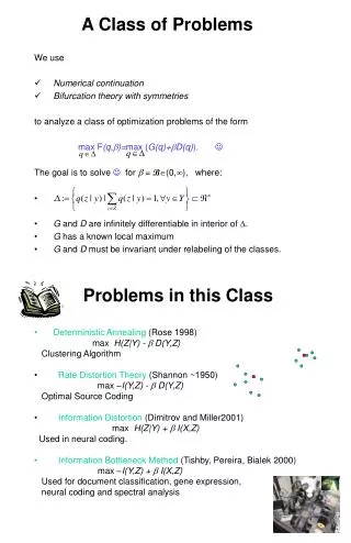
1. A Class of Problems We use • Numerical continuation • Bifurcation theory with symmetries to analyze a class of optimization problems of the form max F(q,)=max (G(q)+D(q)). The goal is to solve  for  = B(0,), where: • . • G and D are infinitely differentiable in interior of . • G has a known local maximum • G and D must beinvariant under relabeling of the classes. Problems in this Class • Deterministic Annealing (Rose 1998) max H(Z|Y) -  D(Y,Z) Clustering Algorithm • Rate Distortion Theory (Shannon ~1950) max –I(Y,Z) -  D(Y,Z) Optimal Source Coding • Information Distortion (Dimitrov and Miller2001) max H(Z|Y) +  I(X,Z) Used in neural coding. • Information Bottleneck Method(Tishby, Pereira, Bialek 2000)max –I(Y,Z) +  I(X,Z) Used for document classification, gene expression, neural coding and spectral analysis

2. p(X) 1 2 3 4 Y X Z is a representation of X using N symbols (or clusters) X 2H(Y) output sequences 2I(X,Y) distinguishable input/output classes of (x,y) pairs Size of an input/output class: 2(H(X|Y) + H(Y|X)) pairs 2H(X) input sequences clustered outputs input source output source Y Z X P(Y |X) q*(Z|Y) Q*(Z |X) Rate Distortion How well is the source X represented by Z? Information Distortion A good communication system has p(X,Y) like: • Goal: Determine the input/output classes of (x,y) pairs. • Idea: We seek to quantize (X,Y) into clusterswhich correspond with the input/output classes. • Method: We determine a quantizer, Q*, between X and Z, a representation of Y using N elements, such that the cost function F(Q*,B)is a maximum for some B (0,).

3. Some nice properties of the problem • The feasible region , a product of simplices, is nice. • Lemma  is the convex hull of vertices (). • When D is convex, the optimal quantizer q* is DETERMINISTIC. • Theorem Theextrema of lie generically on the vertices of .. • Corollary The optimal quantizer is invariant to small perturbations in the model. Solution of the problem when p(X,Y):= 4 gaussian blobs p(X,Y) I(X,Z) vs. N

4. The Dynamical System • Goal: To efficiently solve maxq (G(q) +  D(q))for each , incremented in sufficiently small steps, as   B. • Method: Study the equilibria of the of the flow •  • The Jacobian wrt q of the K constraints {zq(z|y)-1}is J = (IK IK … IK). • The equilibrium at =0 is q*(0)  1/N. • . determines stability and location of • bifurcation. • Assumptions: • Let q*be a local solution to andfixed by SM . • Call the M identical blocks of q F (q*,):B. Call the other N-M blocks of q F (q*,): {R}. • At a singularity (q*,*,*),B has a single nullvector v and Ris nonsingular for every . • If M<N, then BR-1 + MIKis nonsingular. • Theorem: If (q*,*,*) is a bifurcation of equilibria of , then  * 1. • For the four Blob Problem when N >2, the first bifurcation is subcritical (a first order phase transition):

5. Investigating the Dynamical System How: • Use numerical continuation in a constrained system to choose  and to choose an initial guess to find the equilibria q*(). • Use bifurcation theory with symmetriesto understand bifurcations of the equilibria. Continuation • A local maximum qk*(k) of  is an equilibrium of the gradient flow . • Initial condition qk+1(0)(k+1(0)) is sought in the tangent direction  qk , which is found by solving the matrix system • The continuation algorithm used to find qk+1*(k+1) is based on Newton’s method.

6. q* (YN|Y)  Conceptual Bifurcation Structure Bifurcations of q*() Observed Bifurcations for the 4 Blob Problem Bifurcations with symmetry To better understand the bifurcation structure, we use the symmetries of the cost function F(q,). The symmetry is that F(q,) is invariant to relabeling of the N classes of Z The symmetry group of all permutations on N symbols is SN. The action of SN on and q,L (q, ,)is represented by the finite Lie Group whereP is a “block permutation” matrix. The symmetry of is measured by its isotropy group, the subgroup of  which fixes it.

7. What do the bifurcations look like? The Equivariant Branching Lemma gives the existence of bifurcating solutions for every isotropy subgroup which fixes a one dimensional subspace of kerq,L (q*,,). Theorem: Let (q*,*,*) be a singular point of the flow  such that q*is fixed by SM. Then there exists M bifurcating solutions, (q*,*,*) + (tuk,0,(t)), each with isotropy group SM-1, where and v is a nullvector of an unresolved block of the Hessian.  Bifurcation Structure Let T(q*,*) = Pitchform Like Bifurcations. Theorem: All bifurcations “pitchfork like”. Branch Orientation? Theorem: If T(q*,*)> 0,then the branch is supercritical. If T(q*,*)< 0, then the branch is subcritical. Branch Stability? Theorem: If T(q*,*)<0, then all branches fixed by SM-1 are unstable.

8. Partial lattice of the isotropy subgroups of S4 (and associated bifurcating directions) For the 4 blob problem:The isotropy subgroups and bifurcating directions of the observed bifurcating branches isotropy group:S4 S3 S2 1 bif direction:(-v,-v,3v,-v,0)T (-v,2v,0,-v,0)T (-v,0,0,v,0)T …No more bifs!

9. Other Branches The Smoller-Wasserman Theorem ascertains the existence of bifurcating branches for every maximal isotropy subgroup. Theorem: If M is a composite number, then there exists bifurcating solutions with isotropy group <p> for every element  of order M in  and every prime p|M. The bifurcating direction is in the p-1 dimensional subspace of kerq,L (q*,,) which isfixed by <p>. Lattice of the maximal isotropy subgroups <p> in S4 The above theorem states that there are bifurcating solutions from q1/4with symmetry <(1234)2>, <(1243)2>, <(1324)2>. The full lattice of subgroups of the group SM is not known for arbitrary M.

10. A numerical algorithm to solve max F(q,) • Let q0 be the maximizer of maxqG(q), 0=1 and s > 0. For k 0, let (qk , k)be a solution to maxq (G(q) +  D(q)). Iterate the following steps until K= B for some K. • Perform  -step: solve • for and select k+1 =k + dk where • dk = s /(||qk||2 + ||k||2 +1)1/2. • The initial guess for qk+1 at k+1 is qk+1(0) = qk + dk  qk . • Optimization:solve maxq (G(q) + k+1 D(q)) to get the maximizer q*k+1 , using initial guess qk+1(0) . • Check for bifurcation: compare the sign of the determinant of an identical block of each of q [G(qk) + k D(qk)] and q [G(qk+1) + k+1 D(qk+1)]. If a bifurcation is detected, then set qk+1(0) = qk + dku where u is given by  and repeat step 3.