Equilibria in 2D Systems: Types, Stability, and Analysis
290 likes | 325 Vues
This mini-course delves into the equilibria of 2D ODE systems, exploring different types, stability criteria, and analytical methods. Learn how to determine equilibrium types through linearization, eigenvalues, and eigenvectors. Examples, diagrams, and analysis of the Rosenzweig-MacArthur model are included.

Equilibria in 2D Systems: Types, Stability, and Analysis
E N D
Presentation Transcript
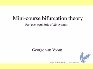
Mini-course bifurcation theory Part two: equilibria of 2D systems George van Voorn
Two-dimensional systems • Consider 2D ODE α = bifurcation parameter(s)
Model analysis • Different kinds of analysis for 2D ODE systems • Equilibria: determine type(s) • Transient behaviour • Long term behaviour
Equilibria: types • Different types of equilibria • Stability • Stable • Unstable • Saddle • Convergence type • Node • Spiral (or focus)
Equilibria: nodes Ws Wu Stable node Unstable node Node has two (un)stable manifolds
Equilibria: saddle Wu Ws Saddle point Saddle has one stable & one unstable manifold
Equilibria: foci Ws Wu Stable spiral Unstable spiral Spiral has one (un)stable (complex) manifold
Equilibria: determination • How do we determine the type of equilibrium? • Linearisation of point • Eigenfunction
Jacobian matrix • Linearisation of equilibrium in more than one dimension partial derivatives
Eigenfunction • Determine eigenvalues (λ) and eigenvectors (v) from Jacobian Of course there are two solutions for a 2D system
Eigenfunction If λ < 0 stable, λ > 0 unstable If twoλ complex pair spiral
Determinant & trace • Alternative in 2D to determine equilibrium type (much less computation)
Diagram Saddle Stable node Stable spiral Unstable spiral Unstable node
Example • 2D ODE Rosenzweig-MacArthur (1963) R = intrinsic growth rate K = carrying capacity A/B = searching and handling C = yield D = death rate
Example • System equilibria • E1 (0,0) • E2 (K,0) • E3 Non-trivial
Example • Jacobian matrix • Substitute the point of interest, e.g. an equilibrium • Determine det(J) and tr(J)
Example Substitution E2 Result: stable node
Example Substitution E3 Result: stable node, near spiral
Example Substitution E3 Result: unstable spiral
One parameter diagram 1 2 3 • Stable node • Stable node/focus • Unstable focus
Isoclines • Isoclines: one equation equal to zero • Give information on system dynamics • Example: RM model
Manifolds & orbits • Manifolds: orbits starting like eigenvectors • Give other information on system dynamics • E.g. discrimination spiral or periodic solution (not possible with isoclines) • Separatrices (unstable manifolds)
Manifolds & orbits y E3 Ws Wu E1 E2 x D < 0 stable manifold E1 is separatrix
Continue • In part three: • Bifurcations in 2D ODE systems • Global bifurcations • In part four: • Demonstration: 3D RM model • Chaos