Understanding Autocatalytic Control in Minimal Metabolic Models
This study delves into minimal metabolic models that explore autocatalytic and control dynamics with a focus on ATP production and intermediate metabolite regulation. It examines feedback mechanisms, trade-offs between robustness and fragility in biological systems, and integrates concepts from thermodynamics, communications, control theory, and computation. By investigating regulatory hard limits and the evolution of complex biological mechanisms, this research aims to provide insights into the necessity versus accident debate in metabolic engineering and system design.

Understanding Autocatalytic Control in Minimal Metabolic Models
E N D
Presentation Transcript
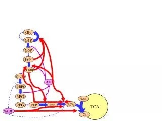
Gly G1P G6P F6P F1-6BP Gly3p ATP 13BPG 3PG TCA Oxa ACA 2PG PEP Pyr NADH Cit
F6P F1-6BP Gly3p ATP 13BPG 3PG Gly G1P G6P F6P F1-6BP Gly3p ATP 13BPG 3PG TCA Oxa ACA 2PG PEP Pyr NADH Cit
Autocatalytic x Control y F6P F1-6BP Gly3p ATP 13BPG 3PG
F6P F1-6BP Gly3p ATP 13BPG 3PG Autocatalytic x Control y
Autocatalytic x Control y Minimal metabolism model • x = ultimate product (ATP) • y = intermediate metabolite • Two feedbacks of x: • Autocatalytic • Control
RHP z and p Hard limits
Autocatalytic x Control y
x produced y consumed
Autocatalytic x Control y consumed produced
x consumed
Autocatalytic x y
Autocatalytic x Control y
Autocatalytic x Control y
1.05 h >>1 h = 1 0.8 h >>1 0.6 Spectrum 0.4 0.2 h = 1 Log(|Sn/S0|) 0 -0.2 -0.4 -0.6 -0.8 0 2 4 6 8 10 Frequency Ideal [ATP] 1 0.95 Time response 0.9 0.85 0.8 0 5 10 15 20 Time (minutes)
1.05 Yet fragile Robust [ATP] 1 h >> 1 0.95 Time response 0.9 0.85 h = 1 0.8 0 5 10 15 20 Time (minutes) 0.8 h >>1 0.6 Spectrum 0.4 0.2 h = 1 Log(Sn/S0) 0 -0.2 -0.4 -0.6 -0.8 0 2 4 6 8 10 Frequency
Yet fragile 0.8 h = 3 0.6 Robust 0.4 0.2 h = 0 Log(Sn/S0) 0 -0.2 -0.4 -0.6 -0.8 0 2 4 6 8 10 Frequency
Yet fragile 0.8 0.6 Robust 0.4 0.2 h = 0 Log(Sn/S0) 0 -0.2 -0.4 -0.6 -0.8 0 2 4 6 8 10 Frequency
This tradeoff is a law. Transients, Oscillations log|S| Biological complexity is dominated by the evolution of mechanisms to more finely tune this robustness/fragility tradeoff. Tighter regulation
Hard limits RHP p RHP z Benefits must be “paid for” within bandwidth z
“Optimal” controller x “Optimal” enzyme y Necessity, not accident
q=α=0 q=α=1 Necessity, not accident 0 10 0 10
Necessity or accident? • Alternative designs Synthesis challenges • Other rates and uncertainty • Computational complexity • Higher order dynamics • Global, nonlinear • Comparisons with data • Robustness is key
Hard limits and tradeoffs Robust/ fragile is unifying concept On systems and their components • Thermodynamics (Carnot) • Communications (Shannon) • Control (Bode) • Computation (Turing/Gödel) • Include dynamics and feedback • Extend to networks • New unifications are encouraging
cost = amplification goal: make this small • benefits = attenuation of disturbance • goal: make this as negative as possible Constraint: benefits costs
Bode d e=d-u - u Plant Control stabilize benefits costs
Bode d e=d-u - u Plant Control Negative is good stabilize benefits costs
Disturbance - e=d-u d Remote Sensor Plant Control Channel Sensor Channel Control Encode Nuno C Martins and Munther A Dahleh, Feedback Control in the Presence of Noisy Channels: “Bode-Like” Fundamental Limitations of Performance. Nuno C. Martins, Munther A. Dahleh and John C. Doyle Fundamental Limitations of Disturbance Attenuation in the Presence of Side Information (Both in IEEE Transactions on Automatic Control) http://www.glue.umd.edu/~nmartins/
Electric power network Variety of producers • Good designs transform/manipulate energy • Subject (and close)to hard limits Variety of consumers
110 V, 60 Hz AC (230V, 50 Hz AC) Gasoline ATP, glucose, etc Proton motive force Standard interface Constraint that deconstrains Variety of consumers Variety of producers Energy carriers
Robust Fragile Disturbance - e=d-u d Remote Sensor Control Channel Plant Sensor Channel Control Encode remote control benefits stabilize remote sensing feedback costs • Robust designs transform/manipulate robustness • Subject (and close) to hard limits • Fragile designs are far away from hard limits and waste robustness.
Hard limits and tradeoffs Robust/ fragile is unifying concept On systems and their components • Thermodynamics (Carnot) • Communications (Shannon) • Control (Bode) • Computation (Turing/Gödel) • Include dynamics and feedback • Extend to networks • New unifications are encouraging
[a system] can have [a property] robust for [a set of perturbations] Fragile Yet be fragile for Robust [a different property] Or [a different perturbation]
[a system] can have [a property] robust for [a set of perturbations] Fragile • Some fragilities are inevitable in robust complex systems. Robust • But if robustness/fragility are conserved, what does it mean for a system to be robust or fragile?
Emergent Fragile • Some fragilities are inevitable in robust complex systems. Robust • But if robustness/fragility are conserved, what does it mean for a system to be robust or fragile? • Robust systems systematically manage this tradeoff. • Fragile systems waste robustness.
Sugars Diverse Fatty acids Precursors Co-factors Catabolism Universal Control Amino Acids Diverse Nucleotides Genes Proteins Carriers Trans* DNA replication Systems requirements: functional, efficient, robust, evolvable Hard constraints: Thermo (Carnot) Info (Shannon) Control (Bode) Compute (Turing) Protocols Constraints Components and materials: Energy, moieties