Download

1 / 22
220 likes | 410 Vues
CFD Modeling of Wind Farms in Flat and Complex Terrain. J. M. Prospathopoulos, E. S. Politis , P. K. Chaviaropoulos K. G. Rados, G. Schepers, D. Cabezon, K. S. Hansen and R. J. Barthelmie. Numerical issues in modeling. Correction of the velocity deficit underestimation in the near wake

E N D
CFD Modeling of Wind Farms in Flat and Complex Terrain J. M. Prospathopoulos, E. S. Politis, P. K. Chaviaropoulos K. G. Rados, G. Schepers, D. Cabezon, K. S. Hansenand R. J. Barthelmie
Numerical issues in modeling • Correction of the velocity deficit underestimation in the near wake • Modification of the turbulence model • Realizability constraint • Definition of the reference wind speed for thrust estimation • Independent of the distance from the W/T rotor • Induction factor concept
Test cases examined • 5 W/T in a row for stable conditions • ECN test wind farm, flat terrain • WT distance = 3.8 D • Wind speed: 6-8 m/s • Wind directions: ±30 degs
Test cases examined • Real wind farm in complex terrain with 43 W/Ts • Complex terrain in Spain, neutral conditions • Distance between rows ≈ 11D • Distance between WTs at the same row ≈ 1.8D • Wind speed 8 m/sWind direction 327 degs
Navier–Stokes modeling • RANS solver based on the pressure correction scheme • Body fitted coordinate transformation • Numerically integration of equations with an implicit multi-block scheme • A matrix-free, conjugate gradient type, solver handles the pressure correction • Developed, used and verified in European research projects (UpWind) • Turbulence model k-ω modified for atmospheric flows • Constants: • Rotor modeling • Momentum sink through actuator force
Boundary conditions • Wind speed profile at inlet • k & ω profiles at inlet
Modeling of stable conditions • Additional buoyancy term is added for turbulence • Add buoyancy term to k and ω equations: • k-equation: • ω-equation: • Dirichlet inflow conditions (common approach): • Neumann inflow conditions (calculate coefficients to satisfy N-S equations): • Similar results
Computational Grids • Horizontal grid spacing 0.05 D close to the W/Ts • Grid refinement in vertical direction close to the ground • 1st grid line 0.01 D above ground • Grid refinement in W/T rotor disk • 21 grid points along rotor diameter
Computational Grids • Minimum grid spacing at xy-plane: 0.08 D / 0.1 D close to the W/Ts • First vertical grid-line at 0.5 m above ground • 100 grid points over the rotor disk area • 7 million grid-points for the total simulation
Turbulence model correction • Velocity deficit underestimation ↔ Turbulence overestimation • Concept from stagnation point flows where turbulence overestimation is also observed • Realizibility constraint for turbulent velocities • Apply the constraint on the eddy viscosity formula in the principal axes of the strain tensor • Relationship for turbulent time scale: • Substitution of the turbulent time scale T in: • Calculation of turbulent viscosity • ω-transport equation
Definition of the reference wind speed • Typical definition: 1 D upstream of the W/T • Mean value over the rotor disk area • Hub height value (centre of the rotor disk) • This stems from isolated W/Ts in flat terrain considerations • Issues that arise: • Is this valid in complex terrain? • Is this valid in wake simulations?
Induction factor concept • Definition of induction factor: • Relationship between CT and induction factor • Iterative procedure starting from an initial guess of Uref
5 W/Ts in flat terrain • Induction factor method: Overestimation of power is in accordance to the single W/T predictions • Under-performance of the 2nd W/T is not reflected in the predictions 1D Upstream Induction factor
5 W/Ts in flat terrain • Predictions performed using induction factor method • Overestimation of W/Ts performance is partially corrected • Under-performance of the 2nd W/T is reproduced by the calculation Baseline model Turbulence model correction
43 W/Ts in complex terrain • “No wakes”: Predictions without W/Ts (terrain effect) • “Flat terrain”: Predictions in flat terrain (1D upstream) • “Terrain+wakes”: Complete simulation (1D upstream)
43 W/Ts in complex terrain • Uncertainty of operational data is related to the lack of calibration for the power converter and yaw position signals. So, the estimation of the reference WT’s yaw position was not better than ±5 degs.
43 W/Ts in complex terrain • “Fine grid”: dx=0.05D, dy=0.07D, dz=0.25m (5 million nodes) • 1D upstream reference wind speed and induction factor taken at hub height
43 W/Ts in complex terrain • 1D upstream reference velocity gives better predictions • Finer discretization improves the results • Fine grids are necessary to simulate complex terrain
Summary • Baseline predictions underestimate near wake deficit • Modeling approaches decrease the turbulence production in the near wake & correct the deficit • Adjustment of additional parameters is needed • Durbin’s correction bounds the turbulent time scale • Based on a general constraint for the turbulent velocities • No adjustment of additional parameters is needed • Reference wind speed is defined through induction factor concept • Applicable on W/Ts located in wakes of neighboring W/Ts
Summary • Durbin’s correction improves the power prediction in a 5 W/Ts wind farm • Induction factor method does not produce satisfactory predictions in complex terrain • Its use should be further investigated
Acknowledgements • This work has been partially financed by the EC within the FP6 UpWind project (# SES6 079945) and by the Greek Secretariat for Research and Technology • The wind farm owners for supplying the data for the model evaluation
Thank you for your attention! • Correspondence to: Evangelos S. Politis Wind Energy Department 19th km Marathonos Avenue, GR19009, Pikermi, Greece Email : vpolitis@cres.gr