CFD Modeling of Turbulent Flows
920 likes | 2.89k Vues
CFD Modeling of Turbulent Flows. Overview. Properties of turbulence Predicting turbulent flows DNS LES RANS Models Summary. u. Time. Properties of Turbulence. Most flows encountered in industrial processes are turbulent.

CFD Modeling of Turbulent Flows
E N D
Presentation Transcript
Overview • Properties of turbulence • Predicting turbulent flows • DNS • LES • RANS Models • Summary
u Time Properties of Turbulence • Most flows encountered in industrial processes are turbulent. • Turbulent flows exhibit three-dimensional, unsteady, aperiodic motion. • Turbulence increases mixing of momentum, heat and species. • Turbulence mixing acts to dissipate momentum and the kinetic energy in the flow by viscosity acting to reduce velocity gradients. • Turbulent flows contain coherent structures that are deterministic events.
Role of Numerical Turbulence Modeling • An understanding of turbulence and the ability to predict turbulence for any given application is invaluable for the engineer. • Examples: • Increased turbulence is needed in chemical mixing or heat transfer when fluids with dissimilar properties are brought together. • turbulence increases drag due to increased frictional forces. • Historically, experimental measurement of the system was the only option available. This makes design optimization incredibly tedious.
Characteristics of the Engineering Turbulence Model • Numerical modeling of turbulence can serve to improve the engineers ability to analyze turbulent flow in design particularly when precise measurements cannot be obtained and when extensive experimentation is costly and time-consuming. • The ideal turbulence model should introduce minimal complexity while capturing the essence of the relevant physics.
Modeling Turbulent Flows • Turbulent flows can be modeled in a variety of ways. With increasing levels of complexity they are: • Correlations • Moody chart, Nusselt number correlations • Integral equations • Derive ODE’s from the equations of motion • Reynolds Averaged Navier Stokes or RANS equations • Average the equations of motion over time • Requires closure • Large Eddy Simulation or LES • Solve Navier-Stokes equations for large scale motions of the flow. Model only the small scale motions • DNS • Navier-Stokes equations solved for all motions in the turbulent flow
Turbulence Modeling Approaches Zero-Equation Models One-Equation Models Two-Equation Models Standard k-e RNG k-e Second-order closure Reynolds-Stress Model Large-Eddy Simulation Direct Numerical Simulation Increase Computational Cost Per Iteration Include More Physics
Direct Numerical Simulation (DNS) • Currently DNS is the most exact approach to modeling turbulence since no averaging is done or approximations are made • Since the smallest scales of turbulence are modeled, called the Kolmogoroff scale, the size of the grid must be scaled accordingly. • A DNS simulation scales with ReL3(u´L/n) where ReL ~ 0.01Re. Turbulent flow past a cylinder would require at least (0.01 x 20,000)3 or 8 million cells
Direct Numerical Simulation (DNS) • Given the current processing speed and memory of the largest computers, only very modest Reynolds number flows with simple geometries are possible. • Advantages: DNS can be used as numerical flow visualization and can provide more information than experimental measurements; DNS can be used to understand the mechanisms of turbulent production and dissipation. • Disadvantages: Requires supercomputers; limited to simple geometries.
Large Eddy Simulation (LES) • LES is a three dimensional, time dependent and computationally expensive simulation, though less expensive than DNS. • LES solves the large scale motions and models the small scale motions of the turbulent flow. • The premise of LES is that the large scale motions or eddies contain the larger fraction of energy in the flow responsible for the transport of conserved properties while the small. DNS u DNS LES LES t
Large Eddy Simulation (LES) • The large scale components of the flow field are filtered from the small scale components using a wavelength criteria related to the size of the eddies • The filter produces the following equation used to model the small scale motions • where • The inequality is then modeled as • tij is called the subgrid scale Reynolds Stress. Different subgrid scale models are available to approximate tij .
Large Eddy Simulation (LES) • Mixing plane between two streams with unequal scalar concentrations • Unsteady vortex motions with growing length scale
Reynolds Averaged Navier-Stokes (RANS) Models • DNS and LES can produce an overwhelming quantity of detailed information about a flow structure. Generally, in engineering flows, such levels on instantaneous information is not required. • Typical engineering flows are focused on obtaining a few quantitative of the turbulent flow. For example, average wall shear stress, pressure and velocity field distribution, degree of mixedness in a stirred tank, etc. • The approach would be to model turbulence by averaging the unsteadiness of the turbulence. • This averaging process creates terms that cannot be solved analytically but must be modeled. • This modeling approach has been around for 30 years and is the basis of most engineering turbulence calculations.
RANS Equations • Velocity or a scalar quantity can be represented as the sum of the mean value and the fluctuation about the mean value as: • Using the above relationship for velocity(let f = u) in the Navier-Stokes equations gives (as momentum equation for incompressible flows with body forces). • TheReynolds Stressescannot be represented uniquely in terms of mean quantities and the above equation is not closed. Closure involves modeling the Reynolds Stresses.
Closure of RANS equations • The RANS equations contain more unknowns than equations. • The unknowns are the Reynolds Stress terms. • Closure Models are: • zero-equation turbulence models • Mixing length model • no transport equation used • one-equation turbulence models • transport equation modeled for turbulent kinetic energy k • two-equation models • more complete by modeling transport equation for turbulent kinetic energy k and eddy dissipation e • second-order closure • Reynolds Stress Model • does not use Bousinesq approximation as first-order closure models
Modeling Turbulent Stresses in Two-Equation Models • RANS equations require closure for Reynolds stresses and the effect of turbulence can be represented as an increased viscosity • The turbulent viscosity is correlated with turbulent kinetic energy k and the dissipation rate of turbulent kinetic energy e Boussinesq Hypothesis: eddy viscosity model Turbulent Viscosity:
Turbulent kinetic energy and dissipation • Transport equations for turbulent kinetic energy and dissipation rate are solved so that turbulent viscosity can be computed for RANS equations. Turbulent Kinetic Energy: Dissipation Rate of Turbulent Kinetic Energy:
Destruction Convection Diffusion Generation Standard k- Model Turbulent Kinetic Energy Dissipation Convection Generation Diffusion Dissipation Rate are empirical constants (equations written for steady, incompressible flow w/o body forces)
Deficiencies of the Boussinesq Approximation • The two-equation models based on the eddy viscosity approximation provide excellent predictions for many flows of engineering interest. • Applications for which the approximation is weak typically are flows with extra rate of strain (due to isotropic turbulent viscosity assumption). Examples of these are: • flows over boundaries with strong curvature • flows in ducts with secondary motions • flows with boundary layer separation • flows in rotating and stratified fluid • strongly three dimensional flows • The RNG k-e model is an improvement over the standard k-e for these classes of flow by incorporating the influence of additional strains rates. • A higher-order closure approximation can be also applied to include wider class of problems including those with extra rates of strain.
Generation Dissipation Diffusion Convection Additional term related to mean strain & turbulence quantities Convection Generation Diffusion Destruction are derived using RNG theory RNG k- Model Turbulent Kinetic Energy where Dissipation Rate (equations written for steady, incompressible flow w/o body forces)
Second-Order Closure models • The Second-Order Closure Models include the effects of streamline curvature, sudden changes in strain rate, secondary motions, etc. • This class of models is more complex and computationally intensive than the RANS models • The Reynolds-Stress Model (RSM) is a second-order closure model and gives rise to 6 Reynolds stress equations and the dissipation equation Reynolds Stress Transport Equation Diffusion Convection Pressure-Strain redistribution Generation Dissipation
Pressure/velocity fluctuations Turbulent transport Reynolds Stress Model Generation (computed) Pressure-Strain Redistribution (modeled) Dissipation (related to e) Turbulent Diffusion (modeled) (equations written for steady, incompressible flow w/o body forces)
Near Wall Treatment • The RANS turbulence models require a special treatment of the mean and turbulence quantities at wall boundaries and will not predict correct near-wall behavior if integrated down to the wall • Special near-wall treatment is required • Standard wall functions • Nonequilibrium wall functions • Two-layer zonal model
Summary • Turbulence modeling comes in varying degrees of complexity. Determining the right choice of turbulence model depends on the detail of results expected. • DNS and LES are still far from being engineering tools but in the near future this will be possible. • Two-equation models are widely used for their relatively simple overhead. However, increased complexity of the turbulent flow reduces the adequacy of the models. • Improvements to the two-equation models to incorporate extra strain rates, and the second-order closure RSM model provide the extra terms to model complex engineering turbulent flows.