Download
1 / 54
720 likes | 2.14k Vues
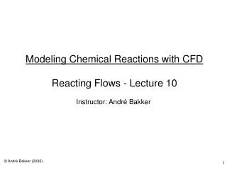
Modeling Chemical Reactions with CFD Reacting Flows - Lecture 10. Instructor: André Bakker. © Andr é Bakker (2006). Outline. Source terms in the species transport equation. Chemical kinetics and reaction rates. Subgrid scale effects. Reaction models and the effects of turbulence.

E N D
Modeling Chemical Reactions with CFD Reacting Flows - Lecture 10 Instructor: André Bakker © AndréBakker (2006)
Outline • Source terms in the species transport equation. • Chemical kinetics and reaction rates. • Subgrid scale effects. • Reaction models and the effects of turbulence. • Examples: • Stirred tank. • Catalytic converter. • Polymerization reactor.
Species transport and reaction • The ith species mass fraction transport equation is: • The mass fraction of chemical species i is Yi. • The velocity is uj. • Di is the diffusion coefficient. • Ri is the reaction source term. Chemical reactions are modeled as source terms in the species transport equation. • Si includes all other sources. Rate of change due to other sources Rate of change due to diffusion Rate of change due to reaction sources Rate of change Net rate of flow (convection) + + = +
Source of species • The net source of chemical species i due to reaction Ri is computed as the sum of the reaction sources over the NR reactions that the species participate in: • Reaction may occur as a volumetric reaction or be a surface reaction. • Note: source terms are also added to the energy equation to take heat of reaction effects into account.
Chemical kinetics • The rth reaction can be written as: • Example:
Reaction rate • The molar reaction rate of creation/destruction of species i in reaction r is given by: • represents the effect of third bodies (e.g. catalysts) on the reaction rate: Here, j,r is the third-body efficiency of the jth species in the rth reaction.
Reaction rate constant • The forward rate constant for reaction r, kf,r is computed using an expanded version of the Arrhenius expression: Ar = pre-exponential factor Er = activation energy R = universal gas constant = 8313 J/kgmol K T = temperature r= temperature exponent • If applicable, the backward rate constant for reaction r, kb,r is computed from the forward rate constant using the relationship: kb,r = kf,r /Kr. • Kr is the equilibrium constant for reaction r, which follows from the thermodynamic properties of the materials.
Reaction rate: the Arrhenius equation • The Arrhenius equation is a formula for the temperature dependence of a chemical reaction rate. Originally it did not include the term T, which was added later by other researchers. • Rk is the Arrhenius reaction rate, E is the activation energy, R is the universal gas constant, and T is the temperature. • First proposed by the Dutch chemist J. H. van 't Hoff in 1884. • Won the 1901 Nobel prize in chemistry for his discovery of the laws of chemical dynamics and osmotic pressure in solutions. • Five years later (1889), the Swedish chemist Svante Arrhenius provided a physical justification and interpretation for it. • Also won the 1903 Nobel prize in chemistry for his electrolytic theory of dissociation and conductivity. • He had proposed that theory in his 1884 doctoral dissertation. It had not impressed his advisors who gave him the very lowest passing grade.
Subgrid effects • For each grid cell the molecular reaction rate can be calculated using the equations presented. • What if there are concentration variations smaller than the size of the grid cell? • Reaction rates calculated at the average concentrations may be overpredicted. • For turbulent flows, models exist that take turbulent mixing effects at subgrid scales into account. Subgrid scale variations
Effect of temperature fluctuations • Temperature may vary in time, and also in space at scales smaller than a grid cell. • What happens if we model a system as steady state and use average temperatures to predict the reaction rates? • Reaction rate terms are highly nonlinear: • Cannot neglect the effects of temperature fluctuations on chemical reaction rates.
Effect of temperature fluctuations - example T 1700 1000 timetrace 300 t • Single step methane reaction (A=2E11, E=2E8): • Assume turbulent fluid at a point has constant species concentration at all times, but spends one third its time at T=300K, T=1000K and T=1700K. • Calculate the reaction rates: • Conclusion: just using the average temperature to calculate reaction rates will give wrong results special reaction models needed.
Laminar finite-rate model • Reaction rates are calculated using the molecular reaction kinetics. • Using average species concentration in cell. • Using average temperature in cell. • No corrections are made for subgrid scale temperature or species concentration variations. • The mesh and, for transient flows, the timestep should be small enough to properly resolve all spatial and temporal variations. • This may lead to very fine mesh and timestep requirements. • If the numerical model is too coarse, species mixing and reaction rates will be overpredicted. Viscous flow with fine striations
Effects of turbulence • In turbulent flows, subgrid and temporal variations in temperature and species concentration are related to the structure of turbulence. • We already solve for the effect of turbulence on the mean flow using turbulence models. • This information can then also be used to predict the effects of turbulence on the reaction rate. • Usually subgrid scale non-uniformities in the species concentration (i.e. poor mixing) result in an effective reaction rate that is lower than the molecular rate kinetics based on average concentrations. • Different reaction models exist for different systems.
Reaction models in FLUENT • Surface reactions: • Particle surface reactions (e.g. coal combustion). • Surface reactions at solid (wall) boundaries (e.g. chemical vapor deposition). • Combustion or infinitely fast chemistry: • Pre-mixed combustion models. • Non pre-mixed combustion models. • Partially pre-mixed combustion models. • Finite-rate kinetics in turbulent flames (composition PDF transport model). • Finite-rate chemistry based on extended Arrhenius equation: • Laminar finite-rate model. • Finite-rate/eddy-dissipation. • Eddy-dissipation. • Eddy-dissipation concept (EDC).
The eddy-dissipation model • A model for the mean reaction rate of species i, Ri based on the turbulent mixing rate. • Assumes that chemical reactions occur much faster than turbulence can mix reactants and heat into the reaction region (Da >> 1). • A good assumption for many combustors: most useful fuels are fast burning. • For fast reactions the reaction rate is limited by the turbulent mixing rate. • The turbulent mixing rate is assumed to be related to the timescale of turbulent eddies that are present in the flow. • Concept originally introduced by Spalding (1971) and later generalized by Magnussen and Hjertager (1976). • The timescale used for this purpose is the so-called eddy lifetime, = k/, with k being the turbulent kinetic energy and the turbulent dissipation rate. • Chemistry typically described by relatively simple single or two step mechanism.
The eddy-dissipation model k - turbulence kinetic energy - turbulence dissipation rate YP, YR - mass fraction of species A - Magnussen constant for reactants (default 4.0) B - Magnussen constant for products (default 0.5) Mw,i - molecular weight (R), (P) - reactants, products • The net rate of production of species i due to reaction r, Ri,r is given by the smaller (i.e. limiting value) of the two expressions below. • Based on mass fraction of reactants: • Based on mass fraction of products: • Here: • Note that kinetic rates are not calculated!
Finite-rate/eddy-dissipation model • The eddy-dissipation model assumes that reactions are fast and that the system is purely mixing limited. • When that is not the case, it can be combined with finite-rate chemistry. • In FLUENT this is called the finite-rate/eddy-dissipation model. • In that case, the kinetic rate is calculated in addition to the reaction rate predicted by the eddy-dissipation model. • The slowest reaction rate is then used: • If turbulence is low, mixing is slow and this will limit the reaction rate. • If turbulence is high, but the kinetic rate is low, this will limit the reaction rate. • This model can be used for a variety of systems, but with the following caveats: • The model constants A and B need to be empirically adjusted for each reaction in each system. The default values of 4 and 0.5 respectively were determined for one and two-step combustion processes. • The model always requires some product to be present for reactions to proceed. If this is not desirable, initial mass fractions of product of 1E-10 can be patched and a model constant B=1E10 used.
Example: parallel competitive reactions • Stirred tank system with parallel-competitive reactions: • Reaction 1 is fast (k1=7300 m3/Mole.s) and reaction 2 is slow (k2=3.5 m3/Mole.s). • The side-product S is only formed in regions with excess B and depleted from A, i.e. poorly mixed regions. • The final product is characteried by the product distribution X: • This indicates which fraction of reactant B was used to create side-product. A lower X indicates less B was used to create side-product.
Using the finite-rate/eddy-dissipation model • This system was previously investigated. • The following Magnussen model constants were determined to give good results for this system: • Reaction 1: model constant A1=0.08. • Reaction 2: model constant A2=1E10. • For both reactions, use model constant B=1E10 and initial product mass fractions of 1E-10 to disable the product mass fraction based reaction rate limiter. • The net effect of this set of model constants is that only the first reaction is limited by mixing rate, but not the second reaction. • The reaction rates were set independent of temperature by specifying zero values for the activation energy and the temperature exponent.
T=0s Mass fraction reactant A Mass fraction reactant B Mass fraction product R Mass fraction product S
T=0.4s Mass fraction reactant A Mass fraction reactant B Mass fraction product R Mass fraction product S
T=0s Reaction rate 1: A + B R Reaction rate 2: B + R S T=0.4s Reaction rate 1: A + B R Reaction rate 2: B + R S
T=2.0s Mass fraction reactant A Mass fraction reactant B Mass fraction product R Mass fraction product S
T=5s Mass fraction reactant A Mass fraction reactant B Mass fraction product R Mass fraction product S
T=2s Reaction rate 1: A + B R Reaction rate 2: B + R S T=5s Reaction rate 1: A + B R Reaction rate 2: B + R S
T=10s Mass fraction reactant A Mass fraction reactant B Mass fraction product R Mass fraction product S
T=20s Mass fraction reactant A Mass fraction reactant B Mass fraction product R Mass fraction product S
T=10s Reaction rate 1: A + B R Reaction rate 2: B + R S T=20s Reaction rate 1: A + B R Reaction rate 2: B + R S
T=40s Mass fraction reactant A Mass fraction reactant B Mass fraction product R Mass fraction product S
Mass fraction reactant A Mass fraction reactant B Mass fraction product R Mass fraction product S
Reaction rate 1 A + B R Reaction rate 2 B + R S
X/Xfinal (Xfinal=0.53) YS/YS,final YR/YR,final YA/YA,initial YB/YB,initial
Other models • The eddy-dissipation-concept (EDC) model. • This is an extension of the eddy-dissipation model to finite rate chemistry; proposed by Gran and Magnussen (1996). • Equations are very different, however. Assumes reactions occur on small scales and calculates a volume fraction of small scale eddies in which the reactions occur. • It is more suitable for more complex reaction sets than the finite-rate/eddy-dissipation model and requires less user tuning. It is computationally expensive, however. • Dedicated combustion models: • Pre-mixed combustion models. • Non pre-mixed combustion models. • Partially pre-mixed combustion models. • Finite-rate kinetics in turbulent flames (composition PDF transport model). • Not standard in FLUENT: reactions for which the kinetics can not practically be described by Arrhenius rate style kinetics. Such kinetics needs to be added through user defined source terms. Examples: • Fermentation kinetics. • Polymerization.
Complex reaction sets • Many real life systems have complex sets of reactions, often many hundreds. • Not all reactions may be known in detail, and there may be uncertainty in the rate constants. • Large differences in time constants may make the reaction set hard (“stiff”) to solve. The reaction sets modeled are usually simplifications of what happens in real life.
Example: catalytic converter • The main component of the catalytic converter is the monolith • The monolith usually has a honeycomb structure, which is coated with one or more catalysts, known as the washcoat (platinum, rhodium, palladium). CO mass fraction Temperature rise due to reaction Catalyst Housing Monolith
Reaction mechanism 61 surface reactions 8 gas phase species 23 surface site species 2 catalysts CH3(S) + Pt(S) → CH2(S) + H(S) CH2(S) + H(S) → CH3(S) + Pt(S) CH2(S) + Pt(S) → CH(S) + H(S) CH(S) + H(S) → CH2(S) + Pt(S) CH(s) + Pt(s) → C(S) + H(S) C(S) + H(S) → CH(S) + Pt(S) C2H3(S) + O(s) → Pt(S) + CH3CO(S) CH3CO(S) + Pt(s) → C2H3(S) + CO(S) CH3(s) + CO(s) → Pt(S) + CH3CO(S) CH3CO(s) + Pt(s) → CH3(S) + CO(s) CH3(S) + OH(S) → CH2(S) + H2O(S) CH2(S) + H2O(S) → CH3(S)+ OH(S) CH2(S) + OH(S) → CH(S) + H2O(S) CH(S) + H2O(S) → CH2(S) + OH(S) CH(S) + OH(S) → C(S) + H2O(S) C(S) + H2O(S) → CH(S) + OH(S) O(S) + H(S) → OH(S) + Pt(S) OH(S) + Pt(S) → O(S) + H(S) H(S) + OH(S) → H2O(S) + Pt(S) H2O(S) + Pt(S) → H(S) + OH(S) OH(S) + OH(S) → H2O(S) + O(S) H2O(S) + O(S) → OH(S) + OH(S) CO(S) + O(S) → CO2 (S) + Pt(S) CO2 (S) + Pt(S) → CO(S) + O(S) C(S) + O(S) → CO(S) + Pt(S) CO(S) + Pt(S) → C(S) + O(S) C3H6 oxidation on Pt Adsorption O2 + Pt(S) + Pt(S) → O(S) + O(S) C3H6 + Pt(S) + Pt(S) → C3H6(S) C3H6 + O(S) + Pt(S) → C3H5(S) + OH(s) H2 + Pt(S) + Pt(S) → H(S) + H(S) H2O + Pt(S) → H2O(S) CO2 + Pt(S) → CO2(S) CO + Pt(S) → CO(S) Desorption O(S) + O(S) → Pt(S) + Pt(S) +O2 C3H6(S) → C3H6 + Pt(S) + Pt(S) C3H5(s) + OH(s) → C3H6 + O(S) + Pt(S) H(S) + H(S) → H2 + Pt(S) + Pt(S) H2O(S) → Pt(S) + H2O CO(S) → CO + Pt(S) CO2 (S) → CO2 + Pt(S) Surface reactions C3H5(S) + 5O(s)→ 5OH(S) + 3C(S) C3H6(S) → C3H5(S) + H(S) C3H5(S) + H(S) → C3H6(S) C3H5(S) + Pt(S) → C2H3(S) + CH2 (S) C2H3(S) + CH2(S) → C3H5(S) + Pt(S) C2H3(S) + Pt(S) → CH3(S) +C(S) CH3(S) + C(S) → C2H3(S) + Pt(S) NO reduction on Pt Adsorption NO + Pt(s) → NO(S) Desorption NO(s) → NO + Pt(s) N(s) + N(s) → N2 + Pt(s) +Pt(s) Surface reactions NO(S) + Pt(S) → N(S) + O(S) N(S) + O(S) → NO(S) + Pt(S) NO reduction & COoxidation on Rh Adsorption O2 + Rh(S) + Rh(S) → O(Rh) + O(Rh) CO + Rh(S) → CO(Rh) NO + Rh(S) → NO(Rh) Desorption O(Rh) + O(Rh) → O2 + Rh(s) + Rh(S) CO(Rh) → CO + Rh(S) NO(Rh) → NO + Rh(S) N(Rh)+ N(Rh) → N2 + Rh(S) + Rh(S) NO/CO Surface reactions CO(Rh) +O(Rh) → CO2 + RH(s) + Rh(s) NO(Rh) + Rh(S) → N(Rh) + O(Rh)
Example: polymerization • Polymerization of ethylene C2H4 into low-density poly-ethylene (LDPE). • LDPE is a plastic resin used to make consumer products such as cellophane wrap, diaper liners, and squeeze bottles. • It is important to be able to predict the properties of the LDPE depending on the precise reaction conditions. • The low density polyethylene process is a complex chain of reactions • It involves many steps and many radicals of different lengths. • It starts with a small amount of initiator mixing with a large amount of monomer (ethylene). • The final product is a polymer (polyethylene) of varying length and structure.
The multi-step polymerization process M = monomer Rx = radical (length x) I = initiator A = initiator radical Px = polymer (length x)
Solution method • Instead of solving species equations for every possible radical or polymer length a mathematical method called the “method of moments” is used. • Introduce moments of radical and dead polymer chains: • Here Rx and Px are the mole fractions of radical and polymer with length x (measured in number of monomers per molecule) respectively. • The moments are used to reduce the reaction set and compute the product characteristics, such as molecular weight distribution. • Energy sources are added to represent the heat of the propagation reaction. • The method of moments is used to derive the molecular weight distribution and polydispersity. • Six additional scalar transport equations are solved for the moments of radicals and polymers.
Simplified polymerization process initiator decomposition chain initiation propagation termination chain transfer to monomer
Polydispersity Zp: this is the ratio of the mass average molecular weight to the number average molecular weight. It indicates the distribution of individual molecular weights in a batch of polymers. Monomer conversion X. Here YM and Y0,M are the final and initial monomer mass fractions respectively. Molecular weight: Number averaged: Mass averaged: Here MWm is the molecular weight of the monomer. Obtaining the product characteristics