Morphological Image Processing
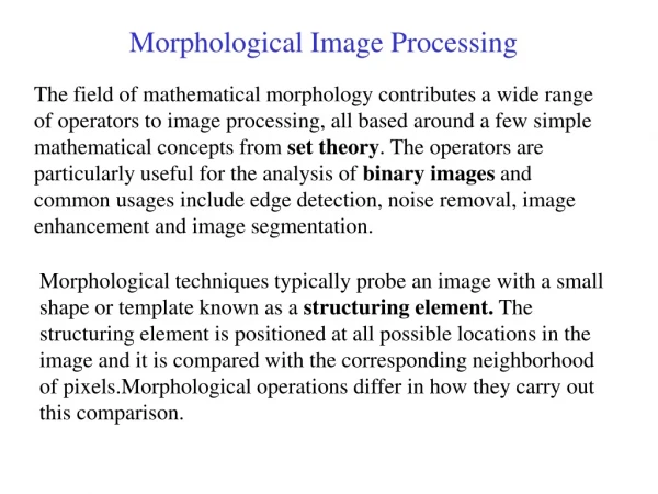
Morphological Image Processing. Morphology. Morphology The branch of biology that deals with the form and structure of organisms without consideration of function Mathematical Morphology Mathematical tool for processing shapes in image, including boundaries, skeletons, convex hulls, etc.

Morphological Image Processing
E N D
Presentation Transcript
Morphology • Morphology • The branch of biology that deals with the form and structure of organisms without consideration of function • Mathematical Morphology • Mathematical tool for processing shapes in image, including boundaries, skeletons, convex hulls, etc. • Use of set theoretical approach (c) 2003-2006 by Yu Hen Hu
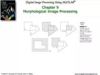
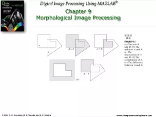
SET () A collection of objects (elements) membership () If is an element (member) of a set , we write Subset () Let A, B are two sets. If for every a A, we also have a B, then the set A is a subset of B, that is, A B If A B and B A, then A = B. Empty set () Complement set If A , then its complement set Ac = {| , and A} Union () A B = {| A or B} Intersection () A B = {| A and B} Set difference (-) B\A = B Ac Note that B-A A-B Disjoint sets A and B are disjoint (mutually exclusive) if A B= Set Theory: Definitions and Notations (c) 2003-2006 by Yu Hen Hu
Set Relations (c) 2003-2006 by Yu Hen Hu
Translation (A)z = { c| c = a + z, for a A } Reflection: Translation and Reflection (c) 2003-2006 by Yu Hen Hu
Logic Operations Between Binary Images (c) 2003-2006 by Yu Hen Hu
Dilation B: structure element Erosion AB = {z | (B)z A} Relations (AB)c = Dilation and Erosion (c) 2003-2006 by Yu Hen Hu
Example of Dilation (c) 2003-2006 by Yu Hen Hu
Example of Erosion (c) 2003-2006 by Yu Hen Hu
Opening A B = (AB) B (c) 2003-2006 by Yu Hen Hu
Closing A B = (AB) B (c) 2003-2006 by Yu Hen Hu
Example: Opening & Closing (c) 2003-2006 by Yu Hen Hu
Finger Print Processing using Opening and Closing (c) 2003-2006 by Yu Hen Hu
Hit-or-Miss Transformation for shape detection (e) (d) Figure 9.12 (a) Set A, (b) A window W and the local Background of X w.r.t. W, W-X. (c) Ac. (d) AX Intersection of (d) and (e) shows the location of the origin of X, as desired. (c) 2003-2006 by Yu Hen Hu
Hit-or-Miss Transform • Denote B1: object, B2: local background of B1, then, or • Reason to have a local background: • Two or more objects are distinct only if they form disjoint (disconnected) sets. This is guaranteed by requiring that each object have at least a one-pixel-thick background around it. (c) 2003-2006 by Yu Hen Hu
Previous example does not contain don’t care entries. In structure element 1 – foreground 0 – background X – don’t care Output is 1 if exact match of both foreground and background pixels. Hitnmiss.m +1: foreground -1: background 0: don’t care Hit-or-Miss Transform Hitnmiss.m (c) 2003-2006 by Yu Hen Hu
Morphological Boundary Extraction (A) = A− (A B) (9.5-1) (c) 2003-2006 by Yu Hen Hu
Example of Boundary Extraction (c) 2003-2006 by Yu Hen Hu
Region Filling Fig915.m (c) 2003-2006 by Yu Hen Hu
Region Filling Example (c) 2003-2006 by Yu Hen Hu
Y: connected component in set A, p: a known point in Y Connected Component Extraction Fig915.m (c) 2003-2006 by Yu Hen Hu
Thinning Thinning is often accomplished using a sequence of rotated structuring elements (a). Given a set A (b), results of thinning with first element is shown in (c), and the next 7 elements (d) – (i). There is no change between 7th and 8th elements, and no change after first 3 elements. Then it converges to a m-connectivity. Fig921.m (c) 2003-2006 by Yu Hen Hu
Thickening AB = A hitnmiss(A,B) A{B} =((…(AB1) B2) … Bn) Thickening is the dual of thinning operation. Usually, thickening a set A is accomplished by thinning Ac, and then complement the result. Then a post-processing prunning process is applied to remove disconnected points as shown to the left. (c) 2003-2006 by Yu Hen Hu
A skeleton of a set A consists of points z that is the center of a maximum disk A maximum disk is a circle in A that can not be enclosed by another circle that is also in A. Figure 9.23. (a) set A, (b), (c) sets of possible maximum disks. (d) dotted line is the skeleton. Skeleton (c) 2003-2006 by Yu Hen Hu
Skeleton Equations • Define k consecutive erosions of A as: AkB = ( …(AB)B) …)B) (9.5-13) Sk(A) = (AkB) − (AkB)B (9.5-12) • Let K = max{k | (AkB) } (9.5-14) Then the skeleton can be found as: (c) 2003-2006 by Yu Hen Hu
Illustration of Skeleton Computation Figure 9.24 Implementation of eq. (9.5-11)-(9.5-15). The original set is at the top left and its morphological skeleton is at the bottom of the 4th column. The reconstructed set is at the bottom of the 6th column. Define k consecutive erosions of A as: AkB = ( …(AB)B) …)B) (9.5-13) Sk(A) = (AkB) − (AkB)B (9.5-12) Let K = max{k | (AkB) } (9.5-14) Then the skeleton can be found as: (c) 2003-2006 by Yu Hen Hu
Pruning (c) 2003-2006 by Yu Hen Hu