Engineering optimization dilemma

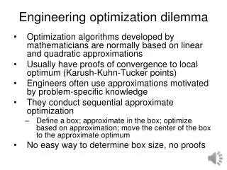
1. Engineering optimization dilemma • Optimization algorithms developed by mathematicians are normally based on linear and quadratic approximations • Usually have proofs of convergence to local optimum (Karush-Kuhn-Tucker points) • Engineers often use approximations motivated by problem-specific knowledge • They conduct sequential approximate optimization • Define a box; approximate in the box; optimize based on approximation; move the center of the box to the approximate optimum • No easy way to determine box size, no proofs

2. Approximation management framework (AMF) • John Dennis at Rice University developed methodology for general approximations for unconstrained problems • His students carried work further for constrained problems • We use paper by two of them (Natalia Alexandrov of NASA Langley and Michael Lewis of the College of William and Mary)

3. Trust region • For approximations, trust region refers to where the approximation is sufficiently accurate. • Some approximations (e.g. Taylor series) can be made very accurate if the region is small enough. • For optimization, a key measure of the accuracy is the ratio between actual and predicted improvement in the objective. • Good improvement ratio means getting the slope approximately right. • Example: If range of values in box is only 5%, any approximation is likely to have small error, but not necessary improvement ratio close to 1.

4. Example • We minimize the function f=1-sinx using the (Taylor series) approximation fa=1-x, starting at x=0. • If our box is |x|<0.5 the solution is x=0.5, f=0.52, fa=0.5. Expected improvement, 0.5, actual improvement 0.48. Improvement ratio is 0.96. Possibly box is too small. • If our box is |x|<1 the solution is x=1, f=0.16, fa=0. Expected improvement, 1, actual improvement 0.84. Looks reasonable • If our box is |x|<2 the solution is x=2, f=0.09, fa=-1. Expected improvement, 2, actual improvement 0.91. Improvement ratio is 0.45. Possibly box is too large • If our box is |x|<4 the solution is x=4, f=1.8, fa=-3. Expected improvement, 4, actual improvement -0.8. Box is too large!

5. Trust region size management algorithm • Optimization in box of function f using approximation fa • Improvement ratio at approximate optimum x* • If r>0 accept new point, otherwise just change box size

6. Box-size algorithm

7. Box-size algorithm

8. Requirement for convergence • For proof of convergence, you need that you can make the error as small as needed by reducing the size of the box. • To satisfy this condition, they modify the approximation near the center of the box using Haftka, R.T., “Combining Global and Local Approximations,” AIAA Journal, Vol. 29, No. 9, pp. 1523-1525, 1991 • The approach creates a hybrid between original approximation and Taylor series approximation near the center, but requires derivatives there.

9. Augmented Lagrangian version • Optimization problem • Augmented Lagrangian • Sub problem: Step 1 • Step 2: Update Lagrange multipliers

10. 3D Wing optimization • Analysis: Euler (CFL3D) • Conditions: • Objective: -L/D • Constraints: lower bound on lift, upper bounds on pitching moment and rolling moment coefficients • Low-fidelity analysis 95x25x17 mesh 8 min. CPU • High fidelity analysis: 193x49x33 mesh, 64min.

11. Comparison of models .

12. Savings Algorithm Improvement. Ratios of savings in function evaluations/derivative calculations (Each low fidelity calculation counts as 1/8 evaluation) Augmented Lagrangian: 3.0/2.6 (kriging) SQP 3.0/3.0 (polynomial) MAESTRO 1.9/1.9 (CFD)