Engineering Optimization

Concepts and Applications Engineering Optimization • Fred van Keulen • Matthijs Langelaar • CLA H21.1 • A.vanKeulen@tudelft.nl

Optimization problem Negative null form Model Definition Checking Recap / overview Special topics Linear / convex problems Sensitivity analysis Topology optimization Solution methods Unconstrained problems Constrained problems Optimality criteria Optimality criteria Optimization algorithms Optimization algorithms

First Order Necessity Condition: • Second Order Sufficiency Condition: H positive definite • For convex f in convex feasible domain: condition for global minimum: • Sufficiency Condition: Summary optimality conditions • Conditions for local minimum of unconstrained problem:

Stationary point nature summary Definiteness H Nature x* Positive d. Minimum Positive semi-d. Valley Indefinite Saddlepoint Negative semi-d. Ridge Negative d. Maximum

Complex eigenvalues? • Question: what is the nature of a stationary point when H has complex eigenvalues? • Answer: this situation never occurs, because H is symmetric by definition. Symmetric matrices have real eigenvalues (spectral theory).

F l k1 k2 Nature of stationary points • Nature of initial position depends on load (buckling):

Nature of stationary points (2)

Unconstrained optimization algorithms • Single-variable methods • 0th order (involving only f ) • 1st order (involving f and f ’ ) • 2nd order (involving f, f ’ and f ” ) • Multiple variable methods

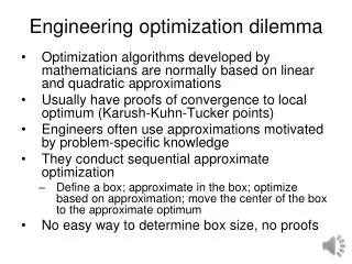
Example: Stationary points: Why optimization algorithms? • Optimality conditions often cannot be used: • Function not explicitly known (e.g. simulation) • Conditions cannot be solved analytically

Weaknesses: • (Usually) less efficient than higher order methods (many function evaluations) 0th order methods: pro/con • Strengths: • No derivatives needed • Work also for discontinuous / non-differentiable functions • Easy to program • Robust

Setting: Iterative process: f Model Optimizer x Minimization with one variable • Why? • Simplest case: good starting point • Used in multi-variable methods during line search

xa xb Termination criteria • Stop optimization iterations when: • Solution is sufficiently accurate (check optimality criteria) • Progress becomes too slow: • Maximum resources have been spent • The solution diverges • Cycling occurs

n points: Final interval size = Ln f x Brute-force approach • Simple approach: exhaustive search • Disadvantage: rather inefficient L0

Basic strategy of 0th order methods for single-variable case • Find interval [a0, b0] that contains the minimum (bracketing) • Iteratively reduce the size of the interval [ak, bk] (sectioning) • Approximate the minimum by the minimum of a simple interpolation function over the interval [aN, bN] • Sectioning methods: • Dichotomous search • Fibonacci method • Golden section method

[a0, b0] x1 x2 = x1+D x3 = x2+gD x4 = x3+g2D Bracketing the minimum f x Starting point x1, stepsize D, expansion parameter g: user-defined

Unimodality • Bracketing and sectioning methods work best for unimodal functions:“An unimodal function consists of exactly one monotonically increasing and decreasing part”

L0 d << L0 a0 b0 L0/2 Dichotomous search Main Entry: di·chot·o·mousPronunciation: dI-'kät-&-m&s also d&-Function: adjective: dividing into two parts • Conceptually simple idea: • Try to split interval in half in each step

Interval size after m steps (2m evaluations): • Proper choice for d : Dichotomous search (2) • Interval size after 1 step (2 evaluations): L0

m Ideal interval reduction Dichotomous search (3) • Example: m = 10

Fibonacci,1180?-1250? x4 x4 Sectioning - Fibonacci • Situation: minimum bracketed between x1 and x3: x1 x2 x3 • Test new points and reduce interval • Optimal point placement?

Optimal sectioning • Fibonacci method: optimal sectioning method • Given: • Initial interval [a0, b0] • Predefined total number of evaluations N,or: • Desired final interval size e

IN IN-2 = 3IN IN-3 = 5IN d << IN IN-4 = 8IN IN-5 = 13IN Fibonacci number Fibonacci sectioning - basic idea • Start at final interval and use symmetry and maximum interval reduction: IN-1 = 2IN

Golden section method uses this constant interval reduction ratio f f 1 f 1 Sectioning – Golden Section • For large N, Fibonacci fraction b converges to golden section ratio f (0.618034…):

I1 I2 = fI1 I2 = fI1 I3 = fI2 • Final interval: Sectioning - Golden Section • Origin of golden section:

Evaluations Example: reduction to 2% of original interval: Ideal dichotomous interval reduction N Dichotomous 12 Golden section 9 Fibonacci 8 (Exhaustive 99) Golden section Fibonacci Comparison sectioning methods • Conclusion: Golden section simple and near-optimal

New point evaluated atminimum of parabola: ai+1 xnew bi+1 Quadratic interpolation • Three points of the bracket define interpolating quadratic function: ai bi • For minimum: a > 0! • Shift xnew when very close to existing point

Cubic interpolation • Similar to quadratic interpolation, but with 2 points and derivative information: ai bi

f’ f Bisection method • Optimality conditions: minimum at stationary point Root finding of f ’ • Similar to sectioning methods, but uses derivative:

Uses linear interpolation f ’ Secant method • Also based on root finding of f ’

Linear approximation • New guess: Newton’s method • Again, root finding of f ’ • Basis: Taylor approximation of f ’:

f’ xk+1 xk+2 xk xk+2 xk xk+1 Newton’s method • Best convergence of all methods: f’ • Unless it diverges

In practice: additional “tricks” needed to deal with: • Multimodality • Strong fluctuations • Round-off errors • Divergence Summary single variable methods • Bracketing + • Dichotomous sectioning • Fibonacci sectioning • Golden ratio sectioning • Quadratic interpolation • Cubic interpolation • Bisection method • Secant method • Newton method 0th order 1st order 2nd order • And many, many more!

Engineering Optimization