1. The Wave Functions
190 likes | 494 Vues
Explore the Schrödinger equation, statistical interpretation, probability, and the uncertainty principle in quantum mechanics. Understand wave functions, normalization, momentum, and more.

1. The Wave Functions
E N D
Presentation Transcript
1. The Wave Functions The Schrodinger Equation The Statistical Interpretation Probability Normalization Momentum The Uncertainty Principle
1.1. The Schrodinger Equation The dynamical state of a particle is completely specified by a wave function . For a non-relativistic, spinless particle, the evolution of (r,t) is governed by the Schrodinger equation Laplacian
Quantization Rule The Schrodinger equation can be obtained by applying the operator rules to the classical relation for a conservative system so that
2. The Statistical Interpretation Born: = Probability amplitude probability of finding particles between a & b at time t. likely to find particle here no chance of finding particle here
Philosophy • Realist (Einstein): There is an objective reality. Causality & locality hold. Statistical nature of quantum theory means that it is incomplete (there are hidden variables). • Orthodox (Copenhagen interpretation / Born ): Statistical nature of measurement is a fundamental property of nature (“strict” causality does not exist). • Agnostic: No need to worry about such metaphysical questions. • Answer to the question: • “Where is the particle just before measurement shows that it is at point C. • Realist : At C. • Orthodox: Nowhere. • Agnostic: Meaningless question. John Bell see p.4 & footnote
Collapse of Wave Function Repeating a measurement right away always gives the same value. Wave function collapses to an eigenfunction of the measurement operator.
3. Probability 3.1. Discrete Variables Let N(j) = number of people whose age is j. In a certain room, N(14) = 1, N(15) = 1, N(16) = 3, N(22) = 2, N(24) = 2, N(25) = 5, N(j) = 0, otherwise Total number of people: Probability of finding a person of age j in room: Probability of finding a person of age j or k : Can always find a person of age between 0 and : Sum rule
Most probable age : 25 (highest probability) Median age : 23 ( 7 people with age below 23; 7 above) Average age : 21 Expectation value Average (expectation) value of a function f of j :
Most probable j = 5. median j = 5. mean j = 5. Variance ( Standard deviation ) :
3.2. Continuous Variables Probability of variable having a value between x and x+dx is (x) dxfor dx 0. probability density. Probability of variable having a value between a and b is
Example 1.1 A rock drops from rest a height h. What is the time average of the distance dropped? Answer: Let x(t) be the distance dropped at time t, with x(T) = h. All time intervals of the same length are the same. Constant acceleration : with
Example 1.1 Alternative Solution Let x be the random variable ( as Griffiths assumed by measuring a million photos ) where
4. Normalization probability of finding particles between a & b at time t. if is finite. ( is square-integrable or normalizable ) Setting and ( is normalized )
Schrodinger Eq. Preserves Normalization if is normalizable ( 0 as |x| )
Equation of Continuity 3D case: Equation of continuity. Conservation of probability. where See Prob. 1.14
5. Momentum Expectation value of x : x average value of x measured on an ensemble of particles in the same state. Reminder: repeated measurements (within a short time interval) on a particle gives only ONE value of x. Integration by part : ( Operator rule for 1st quantization )
In general, any dynamical function f (r, p) in classical mechanics can become a quantum operator by applying the “quantization” rule ( r - representation ) where upon Eg. Full discussion in Chapter 3.
6. The Uncertainty Principle de Broglie formula: If of a particle is a travelling wave of wavelength , the magnitude of the momentum of the particle is = wave number For a wave with a definite , p is definite but x is undefined. For a wave with a small spread in , p is spreaded while x is better defined. For a wave composited of all ’s, p is undefined while x is definite. Uncertainty principle: f= standard deviation of the values of f measured over an ensemble of identically prepared systems.