Large Sample Distribution of EFT and Frequency Domain Techniques for Stationary Processes
This article explores the large sample distribution of the Empirical Fourier Transform (EFT) and its application in analyzing stationary processes. It covers topics such as complex normal theorem, mixing processes, cumulants evaluation, power spectrum estimation, bias correction, and parametric estimation. The text delves into concepts like spectral density matrix, periodogram, crossperiodogram, and prediction models. It also discusses the importance of frequency domain approaches for assessing models and analyzing time-varying variants. Case studies on temperature data, seismic signals, water usage, and spectral analysis techniques are presented.

Large Sample Distribution of EFT and Frequency Domain Techniques for Stationary Processes
E N D
Presentation Transcript
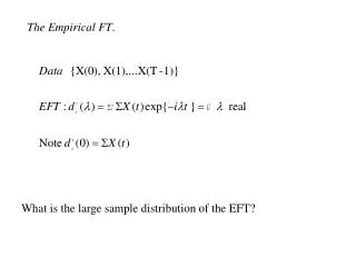
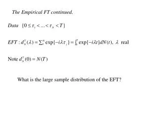
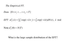
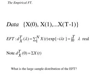
The Empirical FT. What is the large sample distribution of the EFT?
Proof. Write Evaluate first and second-order cumulants Bound higher cumulants Normal is determined by its moments
Comments. Already used to study mean estimate Tapering, h(t)X(t). makes Get asymp independence for different frequencies The frequencies 2r/T are special, e.g. T(2r/T)=0, r 0 Also get asymp independence if consider separate stretches p-vector version involves p by p spectral density matrix fXX( )
Estimation of the (power) spectrum. An estimate whose limit is a random variable
Some moments. The estimate is asymptotically unbiased Final term drops out if = 2r/T 0 Best to correct for mean, work with
Periodogram values are asymptotically independent since dT values are - independent exponentials Use to form estimates
Estimation of finite dimensional . approximate likelihood (assuming IT values independent exponentials)
Crossperiodogram. Smoothed periodogram.
Large sample distributions. var log|AT| [|R|-2 -1]/L var argAT [|R|-2 -1]/L
Berlin and Vienna monthly temperatures
Recife SOI
Partial coherence/coherency. Mississipi dams RXZ|Y = (R XZ – R XZ R ZY )/[(1- |R XZ|2 )(1- |RZY |2 )]
London water usage Cleveland, RB, Cleveland, WS, McRae, JE & Terpenning, I (1990), ‘STL: a seasonal-trend decomposition procedure based on loess’, Journal of Official Statistics Y(t) = S(t) + T(t) + E(t) Seasonal, trend. error
nobs = length(EXP6) # number of observations wsize = 256 # window size overlap = 128 # overlap ovr = wsize-overlap nseg = floor(nobs/ovr)-1; # number of segments krnl = kernel("daniell", c(1,1)) # kernel ex.spec = matrix(0, wsize/2, nseg) for (k in 1:nseg) { a = ovr*(k-1)+1 b = wsize+ovr*(k-1) ex.spec[,k] = mvspec(EXP6[a:b], krnl, taper=.5, plot=FALSE)$spec } x = seq(0, 10, len = nrow(ex.spec)/2) y = seq(0, ovr*nseg, len = ncol(ex.spec)) z = ex.spec[1:(nrow(ex.spec)/2),] # below is text version filled.contour(x,y,log(z),ylab="time",xlab="frequency (Hz)",nlevels=12 ,col=gray(11:0/11),main="Explosion") dev.new() # a nicer version with color filled.contour(x, y, log(z), ylab="time", xlab="frequency(Hz)", main= "Explosion") dev.new() # below not shown in text persp(x,y,z,zlab="Power",xlab="frequency(Hz)",ylab="time",ticktype="detailed",theta=25,d=2,main="Explosion")
Advantages of frequency domain approach. techniques for many stationary processes look the same approximate i.i.d sample values assessing models (character of departure) time varying variant...